Data, vectors and distributions
Lecture 1 (Data Matrix: Vector View) and Lecture 2 (Data Matrix: Probabilistic View), rebuilt as one storyline: first the data as a table of vectors, then one column of that table as a random variable.
How to read this page. It is ordered by concept, not by slide. Every card says which slides it came from, what to read first, and what uses it later. These two lectures are the toolbox that Lectures 3–4 (covariance to PCA) builds on.
Teal = explanation added by Claude, not on the slides. Amber = watch out. Dropdowns hide worked examples, practice questions, and their answers.
The road through the two lectures
Attribute types, linear independence, the median and the IQR are side stops: they appear in the lectures and homework, but the road to PCA does not need them.
Lecture map: which slides each card covers
Part 1
Data as a table
The data matrix: objects and attributes
A dataset is a table. Each row is one thing you measured (a student, a flower) and each column is one measurement (GPA, petal length).
- \(n\)
- number of rows (objects, samples)
- \(m\)
- number of columns (attributes), also called \(d\) in later lectures
- \(x_{ij}\)
- value of attribute \(j\) for object \(i\)
- \(\mathbf x_i\)
- row \(i\) as a column vector in \(\mathbb R^m\)
- \(^T\)
- transpose: turns a row into a column and back
L1 s6 uses bold \(\mathbf x_i\) for row \(i\) (one object) and italic \(\boldsymbol x_j\) for column \(j\) (one attribute). Later lectures (L3 s8, L5 s2, L6 s13) switch between the two. Before any calculation, write down which one you are holding and whether the points are rows or columns.
Running example: the Iris dataset
Every lecture uses Iris for its examples, so remember the shape: 150 rows, 4 numeric columns, one label column that you drop before doing any algebra.
Attribute types: numeric and categorical
Before you compute anything, check what kind of values a column holds. You can add and compare numbers, but you cannot add labels like "male" or "PhD".
| Ask | If yes | If no |
|---|---|---|
| Is it a number you can add? | numeric | categorical |
| Numeric: can it take any value in a range? | continuous | discrete (periodic, binary, counts) |
| Numeric: is zero a true "nothing", so ratios make sense? | ratio-scaled | interval-scaled |
| Categorical: do the values have an order? | ordinal | nominal |
Nominal values can only be tested with \(=\). Writing "male \(\gt\) female" is meaningless. Ordinal values allow \(\lt\) and \(\gt\) but still no arithmetic: PhD \(-\) BS is not a number.
Part 2
Rows as vectors: length, angle, projection, distance
The algebra every later lecture reuses. Lectures 3–4 call it "the algebraic view".
Norm: the length of a vector
The norm is the length of the arrow from the origin to the point. The usual one is the Euclidean norm, which is Pythagoras in \(m\) dimensions.
- \(\|\mathbf x\|\), \(\|\mathbf x\|_2\)
- Euclidean length (the subscript 2 is often dropped)
- \(\mathbf x^T\mathbf x\)
- the vector dotted with itself, equal to the sum of squares
- \(\tilde{\mathbf x}\), \(\mathbf u_x\)
- the unit vector pointing the same way as \(\mathbf x\)
Recipe: normalise a vector
- Square every component and add them up.
- Take the square root. That is the norm.
- Divide every component by the norm. Check: the result has norm 1.
The p-norm family: \(L_1\), \(L_2\), \(L_\infty\)
\(L_1\) is the walking distance along city blocks, \(L_2\) is the straight-line distance, \(L_\infty\) only counts the single biggest step. Changing the norm can change which point is "closest" (see the kNN example under Distance).
The three norms of \(\mathbf x = (1, -2)^T\)
- \[ \|\mathbf x\|_1 = |1| + |-2| = 3 \]
- \[ \|\mathbf x\|_2 = \sqrt{1^2 + (-2)^2} = \sqrt 5 \approx 2.236 \]
- \[ \|\mathbf x\|_\infty = \max\{1, 2\} = 2 \]
- Check the ordering: \(2 \le 2.236 \le 3\) ✓
Norms and unit vectors for two Iris directions
\(\mathbf v_1 = (3.0, 1.1)^T\) and \(\mathbf v_2 = (5.6, 1.4)^T\).
- \[ \|\mathbf v_1\|_2 = \sqrt{3.0^2 + 1.1^2} = \sqrt{10.21} = 3.1953 \]
- \[ \|\mathbf v_2\|_2 = \sqrt{5.6^2 + 1.4^2} = \sqrt{33.32} = 5.7723 \]
- \[ \tilde{\mathbf v}_1 = \frac{\mathbf v_1}{3.1953} = (0.939,\ 0.344)^T \]
- \[ \tilde{\mathbf v}_2 = \frac{\mathbf v_2}{5.7723} = (0.970,\ 0.243)^T \]
L1 s17 prints \(\|\mathbf v_2\| = 5.7728\) and "31953" for 3.1953. The correct value is \(\sqrt{33.32} = 5.7723\); the rest of the slide's numbers are unaffected.
Magnitude of two 5-dimensional vectors
\(V_1 = (1, 2, 3, 4, 5)^T\), \(V_2 = (5, -4, 3, -2, 1)^T\). Calculate the magnitude of each.
- \[ \|V_1\| = \sqrt{1 + 4 + 9 + 16 + 25} = \sqrt{55} = 7.4162 \]
- \[ \|V_2\| = \sqrt{25 + 16 + 9 + 4 + 1} = \sqrt{55} = 7.4162 \]
- Both vectors have the same length.
Inner product and the angle between vectors
The inner product multiplies two vectors position by position and adds up the results. It is large when the vectors point the same way, and it gives you the angle between them.
- \(\langle \mathbf x, \mathbf y \rangle\), \(\mathbf x^T\mathbf y\)
- three notations for the same number
- \(\cos\theta\)
- cosine similarity: \(+1\) same direction, \(0\) perpendicular, \(-1\) opposite
- \(\cos^{-1}\)
- arccos; gives the angle in radians, convert to degrees if asked
Recipe: angle between two vectors
- Compute the dot product.
- Compute both norms.
- \[ \cos\theta = \frac{\text{dot product}}{\text{norm} \times \text{norm}} \]
- \[ \theta = \cos^{-1}(\cos\theta) \] Multiply by \(180/\pi\) for degrees.
The dot product only equals \(\|\mathbf x\|^2\) when \(\mathbf y = \mathbf x\). Mixing up \(\mathbf x^T\mathbf y\) (a number) with \(\mathbf x\mathbf y^T\) (an \(m \times m\) matrix, used in covariance later) is a common slip.
Dot product and angle of \(\mathbf v_1\) and \(\mathbf v_2\)
- \[ \langle \mathbf v_1, \mathbf v_2 \rangle = 3.0 \times 5.6 + 1.1 \times 1.4 = 18.34 \]
- \[ \cos\theta = \frac{18.34}{3.1953 \times 5.7723} = 0.9943 \]
- \[ \theta = \cos^{-1}(0.9943) = 6.1^\circ \]
- The two directions are almost parallel, which matches the Iris plot on the slide.
Semantic search: which document is closest to the query?
Vocabulary (neural, network, recipe). Query \(\mathbf q = (1,1,0)\), documents \(\mathbf d_1 = (2,2,0)\), \(\mathbf d_2 = (6,6,1)\), \(\mathbf d_3 = (0,1,5)\). What should "best match" mean numerically?
- Dot products: \[ \mathbf q^T\mathbf d_1 = 2 + 2 + 0 = 4 \]
- \[ \mathbf q^T\mathbf d_2 = 6 + 6 + 0 = 12 \]
- \[ \mathbf q^T\mathbf d_3 = 0 + 1 + 0 = 1 \]
- Norms: \[ \|\mathbf q\| = \sqrt 2,\quad \|\mathbf d_1\| = \sqrt 8 \]
- \[ \|\mathbf d_2\| = \sqrt{73},\quad \|\mathbf d_3\| = \sqrt{26} \]
- Cosines: \[ \cos\theta_1 = \frac{4}{\sqrt 2 \sqrt 8} = 1.000 \]
- \[ \cos\theta_2 = \frac{12}{\sqrt 2 \sqrt{73}} = 0.993 \]
- \[ \cos\theta_3 = \frac{1}{\sqrt 2 \sqrt{26}} = 0.139 \]
- Euclidean distances: \[ \|\mathbf q - \mathbf d_1\| = \sqrt 2 = 1.414 \]
- \[ \|\mathbf q - \mathbf d_2\| = \sqrt{51} = 7.141 \]
- \[ \|\mathbf q - \mathbf d_3\| = \sqrt{26} = 5.099 \]
- Reading: the raw dot product picks \(\mathbf d_2\) only because it is long (more words). Cosine says \(\mathbf d_1\) points exactly the same way as the query, and \(\mathbf d_2\) almost does. Distance punishes \(\mathbf d_2\) for its length. For text, cosine similarity is the usual choice because it ignores document length.
Dot product, angle and cosine similarity in 5-D
\(V_1 = (1, 2, 3, 4, 5)^T\), \(V_2 = (5, -4, 3, -2, 1)^T\). (a) Dot product. (c) Angle in degrees and cosine similarity. (d) Relation between the vectors.
- \[ V_1^T V_2 = 5 - 8 + 9 - 8 + 5 = 3 \]
- From part (b): \(\|V_1\| = \|V_2\| = \sqrt{55} = 7.4162\).
- \[ \cos\theta = \frac{3}{7.4162 \times 7.4162} = \frac{3}{55} = 0.0545 \]
- \[ \theta = \cos^{-1}(0.0545) = 86.87^\circ \]
- (d) Cosine near 0 and angle near \(90^\circ\): the vectors are nearly orthogonal, and they have the same length.
Read two vectors off a grid, then cosine and angle
From the grid: \(\mathbf u = (3, 4)\), \(\mathbf v = (3, 0)\). Compute the cosine similarity and the angle in degrees.
- \[ \mathbf u \cdot \mathbf v = 3 \times 3 + 4 \times 0 = 9 \]
- \[ \|\mathbf u\| = \sqrt{9 + 16} = 5 \]
- \[ \|\mathbf v\| = \sqrt{9 + 0} = 3 \]
- \[ \cos\theta = \frac{9}{5 \times 3} = 0.6 \]
- \[ \theta = \cos^{-1}(0.6) \approx 53.1^\circ \]
Orthogonal and orthonormal vectors
Two vectors are orthogonal (at right angles) when their dot product is zero. An orthonormal set is a set of unit vectors that are all orthogonal to each other.
The eigenvectors of a covariance matrix form an orthonormal set. That is what lets PCA treat each principal direction separately (see eigen-decomposition).
Checking that \((1,-2,2)\) and \((2,-1,-2)\) are orthogonal
- \[ \mathbf x^T\mathbf y = 1 \times 2 + (-2)(-1) + 2 \times (-2) \]
- \[ \mathbf x^T\mathbf y = 2 + 2 - 4 = 0 \] Orthogonal ✓
Which pairs are orthogonal?
(a) \((2,1,1)\), \((8,2,2)\). (b) \((1,2,3)\), \((2,-2,-3)\). (c) \((1,2,4)\), \((2,1,3)\).
- \[ \text{(a)}\quad 16 + 2 + 2 = 20 \ne 0 \]
- \[ \text{(b)}\quad 2 - 4 - 9 = -11 \ne 0 \]
- \[ \text{(c)}\quad 2 + 2 + 12 = 16 \ne 0 \]
- None of the pairs is orthogonal. (In (a) the second vector is 4 times the first: they are parallel, the opposite of orthogonal.)
Orthogonal projection of one vector onto another
Projecting \(\mathbf y\) onto \(\mathbf x\) means finding the shadow of \(\mathbf y\) along the line of \(\mathbf x\). What is left over is at right angles to \(\mathbf x\).
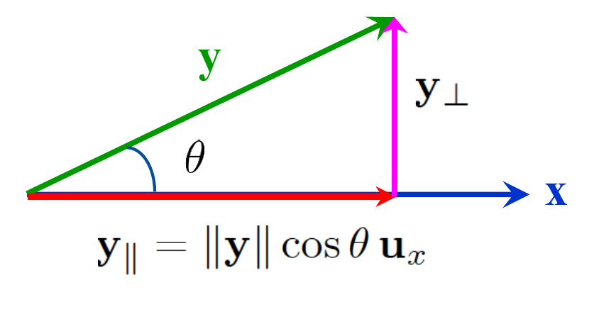
- \(\mathbf y_\parallel\)
- the part of \(\mathbf y\) along \(\mathbf x\) (a vector)
- \(\mathbf y_\perp\)
- the part of \(\mathbf y\) at right angles to \(\mathbf x\): \(\mathbf y - \mathbf y_\parallel\)
- \(\|\mathbf y\|\cos\theta\)
- the scalar projection: the length of the shadow, with a sign
Divide the dot product by \(\|\mathbf x\|^2\), then scale \(\mathbf x\). This is the form the HW1 key and Quiz 1 use. If \(\mathbf x\) is already a unit vector, the shadow length is just \(\mathbf x^T\mathbf y\), which is how PCA computes coordinates (projection onto a basis).
Recipe: project \(\mathbf y\) onto \(\mathbf x\)
- \[ s = \frac{\mathbf x^T\mathbf y}{\mathbf x^T\mathbf x} \]
- \[ \mathbf y_\parallel = s\,\mathbf x \]
- \[ \mathbf y_\perp = \mathbf y - \mathbf y_\parallel \]
- Check: \(\mathbf x^T\mathbf y_\perp = 0\).
"Project \(\mathbf y\) onto \(\mathbf x\)" and "project \(\mathbf x\) onto \(\mathbf y\)" give different vectors: the result always points along the second one. Read the question twice.
Projecting \(\mathbf v_1\) onto \(\mathbf v_2\), the full calculation
\(\mathbf v_1 = (3.0, 1.1)^T\), \(\mathbf v_2 = (5.6, 1.4)^T\).
- \[ \mathbf u_1 = \frac{\mathbf v_1}{3.1953} = (0.9389,\ 0.3443)^T \]
- \[ \mathbf u_2 = \frac{\mathbf v_2}{5.7723} = (0.9701,\ 0.2425)^T \]
- \[ \mathbf v_1^T\mathbf v_2 = 18.34 \]
- \[ \cos\theta = \frac{18.34}{3.1953 \times 5.7723} = 0.9943 \]
- \[ \theta = \cos^{-1}(0.9943) = 6.1^\circ \]
- Scalar projection: \[ \|\mathbf v_1\|\cos\theta = 3.1953 \times 0.9943 = 3.1772 \]
- \[ \mathbf v_{1\parallel} = 3.1772\,\mathbf u_2 = (3.0824,\ 0.7706)^T \]
- \[ \mathbf v_{1\perp} = \mathbf v_1 - \mathbf v_{1\parallel} = (-0.0824,\ 0.3294)^T \]
- \[ \|\mathbf v_{1\perp}\| = \|\mathbf v_1\|\sin\theta = 0.3395 \]
Debiasing word embeddings: remove the component along one direction
Gender direction \(\mathbf g = (3,4)\), \(\|\mathbf g\| = 5\). Occupation vectors \(\mathbf x_{\text{nurse}} = (2,6)\), \(\mathbf x_{\text{eng}} = (0,-5)\). How much of each lies along \(\mathbf g\), and what survives once it is removed?
- Unit direction: \[ \mathbf u_g = \frac{\mathbf g}{5} = (0.6,\ 0.8) \]
- Nurse, scalar projection: \[ \frac{\mathbf x^T\mathbf g}{\|\mathbf g\|} = \frac{6 + 24}{5} = 6 \]
- Nurse, component along \(\mathbf g\): \[ \mathbf x_\parallel = 6\,\mathbf u_g = (3.6,\ 4.8) \]
- Nurse, what survives: \[ \mathbf x_\perp = (2,6) - (3.6, 4.8) = (-1.6,\ 1.2) \] Check: \((-1.6)(3) + (1.2)(4) = 0\) ✓
- Engineer, scalar projection: \[ \frac{0 - 20}{5} = -4 \]
- Engineer, component along \(\mathbf g\): \[ \mathbf x_\parallel = -4\,\mathbf u_g = (-2.4,\ -3.2) \]
- Engineer, what survives: \[ \mathbf x_\perp = (0,-5) - (-2.4,-3.2) = (2.4,\ -1.8) \]
- Reading: "nurse" leans \(+6\) along the gender direction, "engineer" leans \(-4\). Debiasing keeps only \(\mathbf x_\perp\), so both words now have zero component along \(\mathbf g\) and everything else is untouched.
Projection of \(\mathbf u = (3,4)\) onto \(\mathbf v = (3,0)\)
- \[ s = \frac{\mathbf u\cdot\mathbf v}{\|\mathbf v\|^2} = \frac{9}{9} = 1 \]
- \[ \operatorname{proj}_{\mathbf v}(\mathbf u) = 1 \times (3, 0) = (3,\ 0) \]
- Makes sense: \(\mathbf v\) lies on the x-axis, so the shadow of \((3,4)\) is just its x-part.
Projection of \(V_1\) onto \(V_2\) in 5-D
\(V_1 = (1, 2, 3, 4, 5)^T\), \(V_2 = (5, -4, 3, -2, 1)^T\).
- \[ s = \frac{V_1^T V_2}{V_2^T V_2} = \frac{3}{55} = 0.0545 \]
- \[ \operatorname{proj}_{V_2}(V_1) = 0.0545 \times (5, -4, 3, -2, 1)^T \]
- \[ \operatorname{proj}_{V_2}(V_1) = (0.2727,\ -0.2182,\ 0.1636,\ -0.1091,\ 0.0545)^T \]
Distance between two vectors
The distance between two points is the length of the arrow from one to the other. Which norm you use decides what "length" means.
Recipe
- Subtract the two vectors component by component.
- Apply the norm the question asks for (\(L_2\) if it does not say).
Lecture 5 writes the same squared distance as a dot product: \(\|\mathbf x - \mathbf y\|^2 = \mathbf x^T\mathbf x + \mathbf y^T\mathbf y - 2\mathbf x^T\mathbf y\). That identity is what lets kernels compute distances in feature space.
Euclidean and city-block distance between \(\mathbf v_1\) and \(\mathbf v_2\)
- \[ \mathbf v_1 - \mathbf v_2 = (3.0 - 5.6,\ 1.1 - 1.4)^T = (-2.6,\ -0.3)^T \]
- \[ d_2 = \sqrt{(2.6)^2 + (0.3)^2} = \sqrt{6.85} = 2.6173 \]
- \[ d_1 = |-2.6| + |-0.3| = 2.9 \]
k-nearest neighbour on Iris: does the norm change the answer?
Query \(\mathbf q = (4.5, 1.5)\) (petal length, petal width in cm). Candidates \(\mathbf a = (4.8, 1.5)\) [versicolor] and \(\mathbf b = (4.7, 1.7)\) [virginica]. Which is nearer under \(L_2\), \(L_1\), \(L_\infty\)? Does it change if we measure in mm?
- \[ \mathbf q - \mathbf a = (-0.3,\ 0) \]
- \[ \mathbf q - \mathbf b = (-0.2,\ -0.2) \]
- \(L_2\): \[ d(\mathbf q,\mathbf a) = 0.300 \]
- \[ d(\mathbf q,\mathbf b) = \sqrt{0.08} = 0.283 \] Nearest: \(\mathbf b\), virginica.
- \(L_1\): \[ d(\mathbf q,\mathbf a) = 0.3 \]
- \[ d(\mathbf q,\mathbf b) = 0.4 \] Nearest: \(\mathbf a\), versicolor.
- \(L_\infty\): \[ d(\mathbf q,\mathbf a) = 0.3 \]
- \[ d(\mathbf q,\mathbf b) = 0.2 \] Nearest: \(\mathbf b\), virginica.
- In mm every coordinate is multiplied by 10, so every distance is multiplied by 10 and the ranking is unchanged. Scaling only matters when the two attributes are scaled differently.
- Reading: the predicted class depends on the norm. \(L_1\) punishes \(\mathbf b\) for being off in two coordinates; \(L_\infty\) only looks at the worst coordinate.
Linear independence, span, basis and dimension
Vectors are independent when none of them can be built from the others. The number of independent directions you really have is the dimension, which can be smaller than the number of columns.
Put the vectors as columns of a matrix. If one column equals a combination of the others, the vectors are dependent and the rank (true dimension) is less than the number of columns. In PCA, dimension reduction is the same idea: find a small basis that still spans (almost) all of the data.
Redundant sensors: three columns, how many dimensions?
A logger stores intercept (all ones), °C and °F: rows \((1, 20, 68.0)\), \((1, 22, 71.6)\), \((1, 25, 77.0)\), \((1, 21, 69.8)\).
- Check the rule between the columns: \[ 1.8 \times 20 + 32 = 68.0 \]
- \[ 1.8 \times 22 + 32 = 71.6 \] It holds in every row.
- So the °F column is a linear combination of the other two: \[ \mathbf x_{^\circ F} = 1.8\,\mathbf x_{^\circ C} + 32\,\mathbf 1 \]
- In the definition: \(32\,\mathbf x_1 + 1.8\,\mathbf x_2 - 1\,\mathbf x_3 = \mathbf 0\) with non-zero coefficients, so the three columns are dependent.
- Any two of the columns span the same space as all three: the data has 3 columns but only 2 dimensions of information (rank 2). The third column adds nothing new and would make a covariance matrix singular.
Part 3
One attribute as a random variable
Lecture 2 looks at a single column of the data matrix and asks how likely each value is.
An attribute as a random variable
A random variable is a column of the table seen as "a number we did not know until we measured it". It is discrete if it can only take separate values, continuous if it can take any value in a range.
- \(X\)
- capital: the random variable (the idea)
- \(x\), \(x_i\)
- lower case: one observed value
- \(\Pr[\cdot]\)
- probability of an event
Probability mass function (discrete)
For a discrete variable, the pmf is the list of probabilities, one for each possible value. They are each between 0 and 1 and they add up to 1.
Always check the two conditions first. A question that gives you a pmf with an unknown constant is asking you to make the probabilities sum to 1.
Read a pmf and check it
\(p(1) = \frac1{10},\ p(2) = \frac3{10},\ p(3) = \frac2{10},\ p(4) = \frac3{10},\ p(5) = \frac1{10}\). Plot \(p(x)\).
- \[ \tfrac1{10} + \tfrac3{10} + \tfrac2{10} + \tfrac3{10} + \tfrac1{10} = 1 \] Valid pmf ✓
- The plot is five vertical stems at \(x = 1,\dots,5\) with heights 0.1, 0.3, 0.2, 0.3, 0.1, and zero everywhere else. It is symmetric about \(x = 3\).
Cumulative distribution function (discrete)
The cdf at \(x\) is the probability of getting \(x\) or less. For a discrete variable it is a staircase: add up the pmf values as you move right.
Probability of an interval from the cdf: \(\Pr(a \lt X \le b) = F(b) - F(a)\). For a discrete variable, be careful at the endpoints: \(\Pr(a \le X \le b)\) includes \(a\), so subtract \(F\) just below \(a\).
Iris petal length cut into three categories
- Short: \(X \le 2.5\). Medium: \(2.5 \lt X \le 5\). Long: \(X \gt 5\). Code them as \(X \in \{0, 1, 2\}\).
- Count the flowers in each bin: \[ \Pr(\text{Short}) = \tfrac{50}{150} = \tfrac13 \]
- \[ \Pr(\text{Medium}) = \tfrac{58}{150} = 0.3867 \]
- \[ \Pr(\text{Long}) = \tfrac{42}{150} = 0.28 \]
- The cdf steps up at 0, 1, 2: \[ F(0) = 0.3333,\quad F(1) = 0.72,\quad F(2) = 1 \]
Build the cdf from a pmf, then an interval probability
Same pmf as above: \(p(1..5) = 0.1, 0.3, 0.2, 0.3, 0.1\). (b) Compute and plot \(F(x)\). (c) Compute \(\Pr(1.4 \le X \le 4.2)\).
- Running sums: \[ F(1) = 0.1,\quad F(2) = 0.4,\quad F(3) = 0.6 \]
- \[ F(4) = 0.9,\quad F(5) = 1 \]
- \[ F(x) = \begin{cases} 0, & x \lt 1 \\ \sum_{i=1}^{\lfloor x\rfloor} p(i), & 1 \le x \lt 5 \\ 1, & x \ge 5 \end{cases} \] A staircase that jumps at 1, 2, 3, 4, 5.
- (c) The values inside \([1.4, 4.2]\) are 2, 3, 4: \[ \Pr(1.4 \le X \le 4.2) = F(4.2) - F(1.4) = F(4) - F(1) \]
- \[ \Pr = 0.9 - 0.1 = 0.8 \]
Continuous variables: cdf and probability density
A continuous variable has probability zero of hitting any exact value. Instead it has a density: a curve whose area over an interval is the probability of landing in that interval.
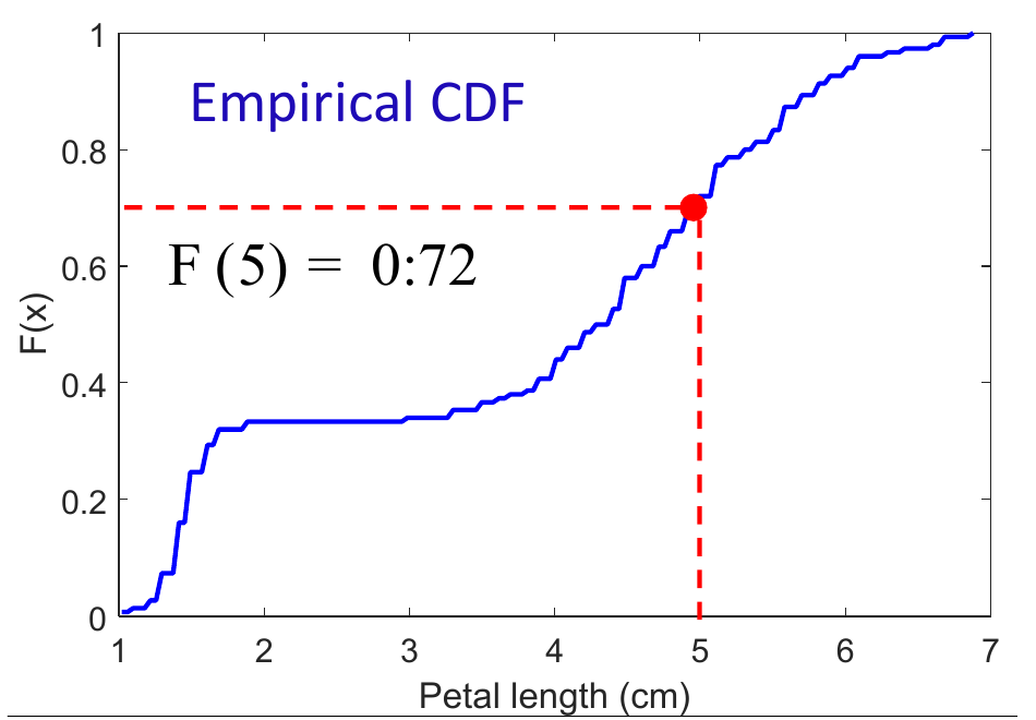
- \(p(x)\), \(f(x)\)
- the density (HW1 writes \(f\))
- \(F(x)\)
- the cdf, area under the density up to \(x\)
- \(\epsilon\)
- a tiny half-width around \(x\)
Recipe: probability of an interval from a density
- If the density has an unknown constant, set the total area to 1 and solve for it.
- Integrate once to get \(F(x)\) (add the "0 below, 1 above" pieces).
- \[ \Pr(a \le X \le b) = F(b) - F(a) \]
For a continuous variable \(\le\) and \(\lt\) give the same answer, because a single point has probability 0. For a discrete variable they do not.
Find the constant, the cdf and an interval probability
\(f(x) = x^2 + \frac23 x + \frac13\) for \(0 \le x \le c\). (a) Find \(c\). (b) Find \(F(x)\). (c) Compute \(\Pr(\frac13 \le X \le \frac23)\).
- Total area must be 1: \[ \int_0^c \Big(x^2 + \tfrac23 x + \tfrac13\Big)dx = \frac{c^3}{3} + \frac{c^2}{3} + \frac{c}{3} \]
- \[ \frac{c^3 + c^2 + c}{3} = 1 \implies c^3 + c^2 + c - 3 = 0 \]
- Try \(c = 1\): \(1 + 1 + 1 - 3 = 0\) ✓. So \(c = 1\). (The cubic has no other positive root: its derivative \(3c^2 + 2c + 1\) is always positive, so it is increasing.)
- \[ F(x) = \begin{cases} 0, & x \lt 0 \\ \frac{x^3 + x^2 + x}{3}, & 0 \le x \le 1 \\ 1, & x \gt 1 \end{cases} \]
- \[ F\!\left(\tfrac23\right) = \frac{\frac{8}{27} + \frac{4}{9} + \frac{2}{3}}{3} = \frac{38}{81} = 0.4691 \]
- \[ F\!\left(\tfrac13\right) = \frac{\frac{1}{27} + \frac{1}{9} + \frac{1}{3}}{3} = \frac{13}{81} = 0.1605 \]
- \[ \Pr\!\left(\tfrac13 \le X \le \tfrac23\right) = \frac{38 - 13}{81} = \frac{25}{81} = 0.3086 \]
Empirical cdf and pmf: estimating from the sample
You never know the true distribution of a column; you estimate it from the rows you have. The empirical cdf at \(x\) is simply the fraction of samples that are at most \(x\).
A hat \(\hat{\ }\) always means "estimated from the sample". The same convention gives \(\hat\mu\), \(\hat\sigma^2\) and \(\hat\Sigma\) below and in Lectures 3–4.
Empirical cdf of five values
\(X = (1.4, 1.4, 1.3, 1.5, 1.4)\), the first five Iris petal lengths. Find \(\hat F(1.4)\).
- Count values \(\le 1.4\): 1.4, 1.4, 1.3, 1.4, that is 4 of 5.
- \[ \hat F(1.4) = \frac45 = 0.8 \]
- The empirical pmf puts mass \(\frac15\) at 1.3, \(\frac35\) at 1.4 and \(\frac15\) at 1.5.
Part 4
Centre and spread of one attribute
Mean and variance feed straight into the mean vector and covariance matrix of Lecture 3. Median, range and IQR are the robust alternatives.
Mean and sample mean
The mean is the balance point of the distribution. The sample mean is the ordinary average of the column, and it is your estimate of the true mean.
- \(E[\cdot]\)
- expectation: a probability-weighted average
- \(\mu_X\)
- the true mean (unknown)
- \(\hat\mu_X\), \(\bar X\)
- the sample mean (computed from data)
The sample mean is the empirical pmf plugged into the discrete formula: each \(x_i\) gets weight \(1/n\). The mean of each column together form the mean vector \(\hat{\boldsymbol\mu}\) of Lecture 3.
Sample mean of a small and a 20-value sample
(i) \(X = (18, 18, 20, 22, 22)\). (ii) \(X\) = (69, 74, 68, 70, 72, 67, 66, 70, 76, 68, 72, 79, 74, 67, 66, 71, 74, 75, 75, 76). Find the sample mean of each.
- \[ \text{(i)}\quad \hat\mu_X = \frac{100}{5} = 20 \]
- \[ \text{(ii)}\quad \sum x_i = 1429 \]
- \[ \hat\mu_X = \frac{1429}{20} = 71.45 \]
Median and why it is robust
The median is the middle value after sorting: half the data sits below it. One wild value can drag the mean a long way, but barely moves the median.
- \(\nu\), \(\hat\nu\)
- median (true, estimated)
- \(F^{-1}\)
- inverse cdf, the quantile function: the \(x\) where the cdf reaches a given level
Sort first. The most common mistake is taking the middle of the unsorted list.
Even and odd samples, and one outlier
- \(X = \{1, 2, 1, 5, 4, 3\}\), sorted \(\{1, 1, 2, 3, 4, 5\}\), \(n = 6\) even: \[ \hat\nu = \tfrac12(2 + 3) = 2.5 \]
- \(X = \{1, 2, 1, 5, 4, 3, 3\}\), sorted \(\{1, 1, 2, 3, 3, 4, 5\}\), \(n = 7\) odd: \[ \hat\nu = x_4 = 3 \]
- \(X = \{1.5, 2, 3.5, 2, 5, 4, 3\}\): \[ \mu = \tfrac{21}{7} = 3 \]
- \[ \nu = 3 \]
- Replace 4 by 32: \(X = \{1.5, 2, 3.5, 2, 5, 32, 3\}\): \[ \mu = \tfrac{49}{7} = 7 \]
- \[ \nu = 3 \] The mean jumped; the median did not move.
Median of the two age samples
- (i) \((18, 18, 20, 22, 22)\) is already sorted, \(n = 5\): the middle value is 20, so the median is 20.
- (ii) Sorted: 66, 66, 67, 67, 68, 68, 69, 70, 70, 71, 72, 72, 74, 74, 74, 75, 75, 76, 76, 79.
- \(n = 20\) even, so average the 10th and 11th: \[ \hat\nu = \frac{71 + 72}{2} = 71.5 \]
- (The key also reports the mode, the most frequent value: 74 appears three times.)
Range, quartiles and the inter-quartile range
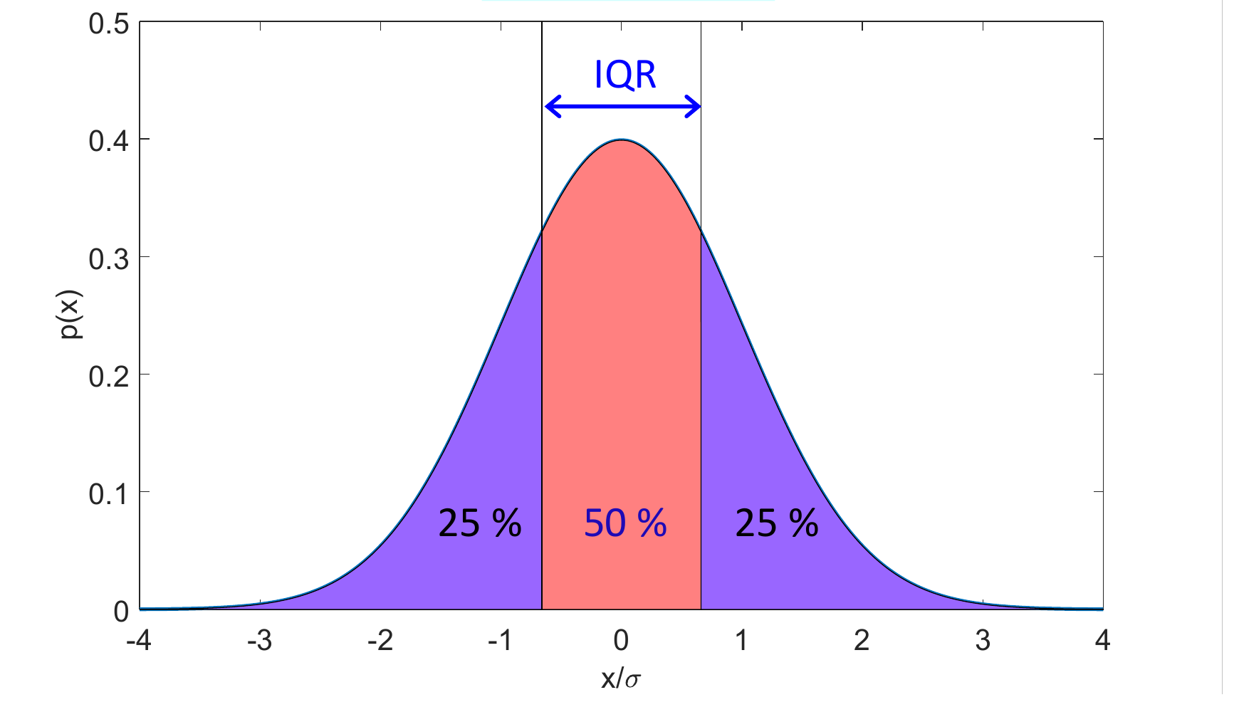
The range is max minus min. The IQR is the width of the middle half of the data, so a single extreme value cannot inflate it.
Computing the quartiles by hand
Software (numpy, Excel) uses other interpolation rules and will give slightly different quartiles. In the exam, follow the slide's method and say which case you used.
Even case: \(X = \{1, 0, -1, 2, -2, 1\}\)
- Sorted: \(\{-2, -1, 0, 1, 1, 2\}\). Lower \(\{-2, -1, 0\}\), upper \(\{1, 1, 2\}\).
- \[ q_1 = \operatorname{median}\{-2, -1, 0\} = -1 \]
- \[ q_3 = \operatorname{median}\{1, 1, 2\} = 1 \]
- \[ IQR = 1 - (-1) = 2 \]
Odd case: \(X = \{1, 0, -1, 2, 2, -2, 1\}\)
- Sorted: \(\{-2, -1, 0, \mathbf 1, 1, 2, 2\}\), median \(= 1\).
- (a) Exclude the median: lower \(\{-2, -1, 0\}\), upper \(\{1, 2, 2\}\). \[ q_1^a = -1 \]
- \[ q_3^a = 2 \]
- (b) Include the median: lower \(\{-2, -1, 0, 1\}\), upper \(\{1, 1, 2, 2\}\). \[ q_1^b = -0.5 \]
- \[ q_3^b = 1.5 \]
- \[ q_1 = \tfrac12(-1 - 0.5) = -0.75 \]
- \[ q_3 = \tfrac12(2 + 1.5) = 1.75 \]
- \[ IQR = 1.75 - (-0.75) = 2.5 \]
All the centre and spread measures for one sample
\(X = \{1, 1, 1.5, 2, 2.5, 3, 4, 5, 7\}\), \(n = 9\).
- \[ \mu = \frac{27}{9} = 3 \]
- Median: already sorted, odd \(n\), the 5th value: \[ \nu = x_5 = 2.5 \]
- Variance (divide by \(n\)): \[ \sigma^2 = \frac{(-2)^2 \times 2 + (-1.5)^2 + (-1)^2 + (-0.5)^2 + 0 + 1^2 + 2^2 + 4^2}{9} \]
- \[ \sigma^2 = \frac{32.5}{9} = 3.6111 \]
- Quartiles, odd case. Excluding the median: lower \(\{1, 1, 1.5, 2\}\) gives \(q_1^a = 1.25\), upper \(\{3, 4, 5, 7\}\) gives \(q_3^a = 4.5\). Including it: lower \(\{1, 1, 1.5, 2, 2.5\}\) gives \(q_1^b = 1.5\), upper \(\{2.5, 3, 4, 5, 7\}\) gives \(q_3^b = 4\).
- \[ q_1 = \frac{1.25 + 1.5}{2} = 1.375 \]
- \[ q_3 = \frac{4.5 + 4}{2} = 4.25 \]
- \[ R = 7 - 1 = 6 \]
- \[ IQR = 4.25 - 1.375 = 2.875 \]
- Outlier fences at \(1.5 \times IQR\) beyond the quartiles: \[ 1.375 - 1.5 \times 2.875 = -2.9375 \]
- \[ 4.25 + 1.5 \times 2.875 = 8.5625 \] Both 1 and 7 are inside, so there are no outliers.
Repeat with the last value 7 replaced by 16
\(X = \{1, 1, 1.5, 2, 2.5, 3, 4, 5, 16\}\). Find the mean, median, variance, quartiles, range, IQR, and check for outliers.
- \[ \mu = \frac{36}{9} = 4 \] (was 3: the mean moved.)
- \[ \nu = x_5 = 2.5 \] (unchanged.)
- \[ \sigma^2 = \frac{176.5}{9} = 19.61 \] (was 3.61: the variance exploded.)
- Quartiles: the lower groups are unchanged, so \(q_1 = 1.375\). Upper groups \(\{3, 4, 5, 16\}\) and \(\{2.5, 3, 4, 5, 16\}\) still have medians 4.5 and 4, so \(q_3 = 4.25\).
- \[ R = 16 - 1 = 15 \] (range tripled.)
- \[ IQR = 2.875 \] (unchanged.)
- Upper fence \(4.25 + 1.5 \times 2.875 = 8.5625\): the value 16 is above it, so it is an outlier. Median and IQR are robust; mean, variance and range are not.
Variance, standard deviation and the sample variance
Variance is the average squared distance from the mean, so it measures spread. Its square root, the standard deviation, is in the same units as the data.
- \(\sigma_X^2\), \(\sigma_X\)
- true variance and standard deviation
- \(\hat\sigma^2\), \(s^2\)
- sample variance (divide by \(n\)) and the unbiased version (divide by \(n-1\))
- \(\tilde{\boldsymbol x}\)
- the centred column: every value minus the mean
Recipe: sample variance by hand
- Compute the mean.
- Subtract it from every value (the centred vector).
- Square each, add up.
- Divide by \(n\) (or \(n-1\) if the question says so). Square root for the standard deviation.
Lectures and HW2 use \(\frac1n\) (the ML estimator). Your practice sheet notes Q3 and the HW1 key for Q3(c) effectively use \(n-1\). Use what the question says; if it says nothing, use \(\frac1n\) and state it.
Variance is a norm, and covariance (Lecture 3) is a dot product of two centred columns. All of Part 2 applies to data columns, not just to points. The variance of every column together gives the diagonal of the covariance matrix.
Sample variance of a weight column
(i) \(Y = (46, 50, 54, 58, 62)\), use \(n-1\). (ii) \(Y\) = (153, 175, 155, 135, 172, 150, 115, 137, 200, 130, 140, 265, 185, 112, 140, 150, 165, 185, 210, 220), use \(n\).
- \[ \text{(i)}\quad \bar Y = \frac{270}{5} = 54 \]
- Deviations \((-8, -4, 0, 4, 8)\), squares sum to 160: \[ s_Y^2 = \frac{160}{4} = 40 \]
- \[ \text{(ii)}\quad \hat\mu_Y = \frac{3294}{20} = 164.70 \]
- \[ \sum (y_i - 164.7)^2 = 27384.2 \]
- \[ \hat\sigma_Y^2 = \frac{27384.2}{20} = 1369.21 \]
- \[ \hat\sigma_Y = \sqrt{1369.21} = 37.00 \] With \(n-1\): 1441.27.
Use the sample mean and standard deviation in a normal model
Age \(X\) (the 20 values above) has \(\hat\mu_X = 71.45\). Assuming \(X\) is normal with the sample mean and sample standard deviation, what is the probability of an age of 80 or higher? (The normal cdf \(\Phi\) is on the z-score card.)
- \[ \sum (x_i - 71.45)^2 = 276.95 \]
- \[ \hat\sigma_X^2 = \frac{276.95}{20} = 13.8475 \]
- \[ \hat\sigma_X = \sqrt{13.8475} = 3.7212 \]
- \[ z = \frac{80 - 71.45}{3.7212} = 2.30 \]
- \[ \Pr(X \ge 80) = 1 - \Phi(2.30) = 1 - 0.9893 = 0.0107 \]
- With the \(n-1\) standard deviation (3.818): \(z = 2.24\), \(\Pr = 0.0126\). Either is about 1%.
The posted HW1 key writes \(\Pr(X \ge 80) = 0\). That is the empirical answer (no sampled age reaches 80), not the normal-model answer the question asks for. Under the normal model the probability is about 0.011. Show the z-score and the table lookup; that is what earns the marks.
Part 5
Exam toolkit
Which formula, when
The formulas are given in the exam. The skill being tested is picking the right one and showing each step.
| The question asks for… | Use | Card |
|---|---|---|
| length / magnitude of a vector | \(\|\mathbf x\| = \sqrt{\mathbf x^T\mathbf x}\) | Norm |
| a unit vector | \(\mathbf x / \|\mathbf x\|\) | Norm |
| \(L_1\) or \(L_\infty\) norm | sum of \(|x_i|\), or the largest \(|x_i|\) | p-norms |
| dot product | \(\sum x_i y_i\) | Inner product |
| cosine similarity / angle | \(\cos\theta = \mathbf x^T\mathbf y / (\|\mathbf x\|\|\mathbf y\|)\) | Inner product |
| are they orthogonal? | check \(\mathbf x^T\mathbf y = 0\) | Orthogonality |
| projection of \(\mathbf y\) onto \(\mathbf x\) | \(\frac{\mathbf x^T\mathbf y}{\mathbf x^T\mathbf x}\,\mathbf x\) | Projection |
| the part left over after projecting | \(\mathbf y - \mathbf y_\parallel\) | Projection |
| distance between two points | \(\|\mathbf x_1 - \mathbf x_2\|\) with the stated norm | Distance |
| are the columns independent? true dimension? | look for one column as a combination of the others | Basis |
| is this a valid pmf? | each \(0 \le p \le 1\), sum \(= 1\) | pmf |
| cdf of a discrete variable | running sum of the pmf | cdf |
| probability of an interval | \(F(b) - F(a)\) | cdf pdf |
| the constant in a density | set \(\int f = 1\) | |
| cdf from a density | \(F(x) = \int_{-\infty}^x f\) | |
| fraction of samples \(\le x\) | \(\hat F(x) = \frac1n \sum I(x_i \le x)\) | Empirical |
| mean of a sample | \(\frac1n \sum x_i\) | Mean |
| mean of a distribution | \(\sum x\,p(x)\) or \(\int x\,p(x)\,dx\) | Mean |
| median | sort, take the middle (average the two middles if \(n\) is even) | Median |
| quartiles, IQR | medians of the lower and upper halves | IQR by hand |
| variance, standard deviation | \(\frac1n\sum(x_i - \hat\mu)^2\), then square root | Variance |
| a probability under a normal model | \(z = (x - \hat\mu)/\hat\sigma\), then the \(\Phi\) table | Variance (then Lectures 3–4, z-score) |