From covariance to PCA

Lecture 3 (Bivariate & Multivariate Analysis) and Lecture 4 (PCA), rebuilt as one storyline: each idea comes before the ideas that need it.

How to read this page. It is ordered by concept, not by slide. Lecture 4 repeats eight slides from Lecture 3; here each idea appears once. Every card says which slides it came from, what it needs, and what uses it.

Teal = explanation added by Claude, not on the slides. Amber = watch out. Dropdowns hide worked examples, practice questions, and their answers.

The road to PCA

Data matrix→Mean→Covariance matrix→Eigen-decomposition→Total variance→Projection→Best direction→PCA algorithm

Correlation and the normal distribution are side branches: they are in the lectures and homework, but PCA does not need them.

Lecture map: which slides each card covers

Part 1

Data as random vectors

Random vectors and the data matrix

Your data is a table: each row is one sample (one flower) and each column is one measurement (like petal length). That table is called the data matrix.

A bivariate random variable is a vector with two component RVs:

\[ \mathbf X = \begin{bmatrix} X_1 \\ X_2 \end{bmatrix} \]

An observed value of it is a vector in \(\mathbb R^2\):

\[ \mathbf x = \begin{bmatrix} x_1 \\ x_2 \end{bmatrix} \]

Example (Iris): \(X_1\) = petal length, \(X_2\) = petal width.

\[ \mathbf x = (1.4,\ 0.2)^T \]

With \(m\) attributes and \(n\) samples, the \(n \times m\) data matrix is

\[ \mathbf X = \begin{bmatrix} x_{11} & x_{12} & \cdots & x_{1m} \\ x_{21} & x_{22} & \cdots & x_{2m} \\ \vdots & & & \vdots \\ x_{n1} & x_{n2} & \cdots & x_{nm} \end{bmatrix} \]

\(n\): number of samples (rows)
\(m\): number of attributes (columns)
\(x_{ij}\): value of attribute \(j\) for sample \(i\)
\(\mathbf X\), \(X_j\): capital letters: the random variable (the idea)
\(\mathbf x\): lower case: observed numbers
hat \(\hat{\ }\): estimated from the sample, e.g. \(\hat{\boldsymbol\mu}\), \(\hat\Sigma\)

L3 s8 writes \(\mathbf X = [\mathbf x_1 \cdots \mathbf x_m]\), where each \(\mathbf x_j\) is a column (one attribute).

L4 s20 writes \(\mathbf X = [\mathbf x_1, \dots, \mathbf x_n]^T\), where each \(\mathbf x_i\) is a row (one sample).

HW2 Q2 and Quiz 2 give points as columns. Always rewrite the data as rows = samples first.

Joint distributions: pmf, cdf, pdf

A joint distribution tells you how likely each combination of values is, for example a petal that is both 4.5 long and 1.5 wide.

Discrete RVs, joint probability mass function:

\[ p(\mathbf x) = \Pr(X_1 = x_1,\ X_2 = x_2) \]

Joint cdf, for all \(\mathbf x \in \mathbb R^2\):

\[ F(\mathbf x) = \Pr(X_1 \le x_1,\ X_2 \le x_2) \]

Continuous RVs, joint pdf:

\[ p(\mathbf x) = \frac{\partial^2 F(x_1,x_2)}{\partial x_1 \partial x_2} \]

Probability of landing in a 2-D area \(\mathcal A\):

\[ \Pr(\mathbf X \in \mathcal A) = \int_{\boldsymbol\xi \in \mathcal A} p(\boldsymbol\xi)\, d\boldsymbol\xi \]

The pdf as probability per unit area:

\[ p(\mathbf x) = \frac{\Pr\{X_1 \in (x_1-\epsilon, x_1+\epsilon],\ X_2 \in (x_2 - \epsilon, x_2+\epsilon]\}}{(2\epsilon)^2} \]

The same definitions extend to more than two variables.

Probability inside a tiny square around \(\mathbf x\), divided by the square's area. (Strictly, as \(\epsilon \to 0\); the slide leaves the limit out.)

Independence and marginals

Two variables are independent when knowing one tells you nothing about the other. Then any joint probability is just the two separate probabilities multiplied.

\(X_1, X_2\) are independent if, for every pair of intervals \(I_1, I_2\):

\[ \Pr(X_1 \in I_1 \text{ and } X_2 \in I_2) = \Pr(X_1 \in I_1) \times \Pr(X_2 \in I_2) \]

If they are independent, then all of these hold:

\[ F(\mathbf x) = F_1(x_1)\,F_2(x_2) \] \[ p(\mathbf x) = p_1(x_1)\,p_2(x_2) \] \[ E[g(X_1)\,h(X_2)] = E[g(X_1)]\,E[h(X_2)] \] \[ \operatorname{Var}(X_1+X_2) = \operatorname{Var}(X_1) + \operatorname{Var}(X_2) \]

The marginal pdfs (“integrate out” the other variable):

\[ p_1(x_1) = \int_{-\infty}^{\infty} p(x_1,x_2)\,dx_2 \] \[ p_2(x_2) = \int_{-\infty}^{\infty} p(x_1,x_2)\,dx_1 \]

Checking independence from a small table

\(X_1, X_2 \in \{0,1\}\) with this joint table:

\[ \begin{array}{c|cc} & X_2 = 0 & X_2 = 1 \\ \hline X_1 = 0 & 0.2 & 0.2 \\ X_1 = 1 & 0.3 & 0.3 \end{array} \]

Marginal of \(X_1\): add along each row. \[ p_1(0) = 0.2 + 0.2 = 0.4 \]
\[ p_1(1) = 0.3 + 0.3 = 0.6 \]
Marginal of \(X_2\): add down each column. \[ p_2(0) = 0.2 + 0.3 = 0.5 \]
\[ p_2(1) = 0.2 + 0.3 = 0.5 \]
Multiply the marginals for one cell. \[ p_1(0)\,p_2(0) = 0.4 \times 0.5 = 0.2 \]
Compare with the table: \(p(0,0) = 0.2\). It matches ✓
Check the others the same way. All four match, so they are independent. One failing cell would make them dependent.

Part 2

Center and spread

Mean vector and total variance

The mean vector is the average of each column. Total variance adds up how spread out each column is, giving one number for the whole data.

The mean of a vector RV is the vector of the component means:

\[ \begin{aligned} \boldsymbol\mu &= E[\mathbf X] \\ &= \begin{bmatrix} E\{X_1\} \\ E\{X_2\} \end{bmatrix} \\ &= \begin{bmatrix} \mu_1 \\ \mu_2 \end{bmatrix} \end{aligned} \]

The sample mean:

\[ \hat{\boldsymbol\mu} = \frac1n \sum_{i=1}^n \mathbf x_i \]

Total variance is the sum of the component variances (same for sample variances):

\[ \sigma^2_{\mathbf X} = \sigma^2_{X_1} + \sigma^2_{X_2} \]

\[ \hat\sigma_j^2 = \frac1n \sum_{i=1}^n (x_{ij} - \hat\mu_j)^2 \]

Subtract the mean, square, then average.

The lectures divide by \(n\) (L3 s7–8, L4 s20), and HW2 says “use \(1/n\)”. Your practice sheet (Q3) used \(n-1\).

Use what the question says. If it says nothing, use \(1/n\).

Mean of 5 Iris-versicolor flowers

Petal length \(X_1 = (4.7, 4.5, 4.9, 4.0, 4.6)\). Petal width \(X_2 = (1.4, 1.5, 1.5, 1.3, 1.5)\).

\[ \hat{\boldsymbol\mu} = \frac15 \begin{bmatrix} 22.7 \\ 7.2 \end{bmatrix} \] \[ \hat{\boldsymbol\mu} = \begin{bmatrix} 4.54 \\ 1.44 \end{bmatrix} \]

Mean, median and variance, small sample

\(X = (18,18,20,22,22)\) (age), \(Y = (46,50,54,58,62)\) (weight). Use \(n-1\). Find the mean and median of \(X\), and the sample variance of \(Y\).

\[ \bar X = \frac{100}{5} = 20 \]
Sorted, the middle value is 20, so the median is 20.
\[ \bar Y = \frac{270}{5} = 54 \]
Deviations of \(Y\): \((-8,-4,0,4,8)\). Their squares add up to 160.
\[ s_Y^2 = \frac{160}{4} = 40 \]

Mean, median, variance, n = 20

\(X\) = (69, 74, 68, 70, 72, 67, 66, 70, 76, 68, 72, 79, 74, 67, 66, 71, 74, 75, 75, 76)

\(Y\) = (153, 175, 155, 135, 172, 150, 115, 137, 200, 130, 140, 265, 185, 112, 140, 150, 165, 185, 210, 220)

\[ \hat\mu_X = \frac{1429}{20} = 71.45 \]
Sorted \(X\): the 10th and 11th values are 71 and 72. \[ \text{median} = \frac{71 + 72}{2} = 71.5 \]
\[ \hat\mu_Y = \frac{3294}{20} = 164.70 \]
\[ \sum (y_i - \hat\mu_Y)^2 = 27384.2 \]
\[ \hat\sigma_Y^2 = \frac{27384.2}{20} = 1369.21 \] With \(n-1\) instead: 1441.27.

Covariance of two variables

Covariance tells you if two variables tend to go up together (positive), move in opposite directions (negative), or have no clear pattern (near zero).

\[ \sigma_{12} = E[(X_1-\mu_1)(X_2-\mu_2)] \]

An equivalent form:

\[ \sigma_{12} = E[X_1X_2] - \mu_1\mu_2 \]

Symmetric: \(\sigma_{12} = \sigma_{21}\).
If \(X_1, X_2\) are independent, then \(\sigma_{12} = 0\).

Sample covariance between two data columns:

\[ \hat\sigma_{12} = \frac1n \sum_{i=1}^n (x_{1i} - \hat\mu_1)(x_{2i} - \hat\mu_2) \]

The same thing in vector form, with \(\mathbf 1 = [1\ 1\ \cdots\ 1]^T\):

\[ \hat\sigma_{12} = \frac1n (\mathbf x_1 - \mathbf 1\hat\mu_1)^T(\mathbf x_2 - \mathbf 1 \hat\mu_2) \]

\(\mathbf x_1 - \mathbf 1\hat\mu_1\) means “subtract the mean from every entry of column 1”. The covariance is the dot product of the two centered columns, divided by \(n\).

Recipe

Compute both means.
Subtract each mean from its own column.
Multiply the centered values row by row.
Add the products and divide by \(n\).

Three data points

\(\mathbf x_1 = [1\ 0\ 2]^T\) with \(\hat\mu_1 = 1\). \(\mathbf x_2 = [0.5\ {-0.5}\ 1.5]^T\) with \(\hat\mu_2 = 0.5\).

\[ \mathbf x_1 - \mathbf 1\hat\mu_1 = [0\ {-1}\ 1]^T \]
\[ \mathbf x_2 - \mathbf 1\hat\mu_2 = [0\ {-1}\ 1]^T \]
\[ \sigma_{12} = \frac13 \begin{bmatrix} 0 & -1 & 1 \end{bmatrix} \begin{bmatrix} 0 \\ -1 \\ 1 \end{bmatrix} \]
\[ \sigma_{12} = \frac13(0 + 1 + 1) \]
\[ \sigma_{12} = \frac23 \]

The covariance matrix

The covariance matrix is one table that holds every variance (on the diagonal) and every covariance (off the diagonal).

For \(\mathbf X = [X_1\ X_2\ \cdots\ X_m]^T\), an \(m\times m\) symmetric positive semidefinite matrix:

\[ \Sigma = E[(\mathbf X - \boldsymbol\mu)(\mathbf X-\boldsymbol\mu)^T] \]

Written out:

\[ \Sigma = \begin{bmatrix} \sigma_1^2 & \sigma_{12} & \cdots & \sigma_{1m} \\ \sigma_{21} & \sigma_2^2 & \cdots & \sigma_{2m} \\ \vdots & \vdots & \ddots & \vdots \\ \sigma_{m1} & \sigma_{m2} & \cdots & \sigma_m^2 \end{bmatrix} \]

Sample covariance matrix:

\[ \hat\Sigma = \frac1n (\mathbf X - \mathbf 1\hat{\boldsymbol\mu}^T)^T (\mathbf X - \mathbf 1 \hat{\boldsymbol\mu}^T) \]

\(\mathbf X - \mathbf 1\hat{\boldsymbol\mu}^T\) means “subtract the mean row from every row”. Lecture 4 calls this centered data \(\mathbf Z\):

\[ \hat\Sigma = \frac1n \mathbf Z^T\mathbf Z \]

Each entry is one column of \(\mathbf Z\) dotted with another, divided by \(n\):

\[ \hat\Sigma_{jk} = \frac1n\,(\text{col } j \text{ of } \mathbf Z)\cdot(\text{col } k \text{ of } \mathbf Z) \]

“Positive semidefinite” just means the spread in any direction is never negative.

Recipe

Write the data as \(n\times m\), with rows = samples.
Compute the mean of every column.
Subtract the mean row from every row. Each column of \(\mathbf Z\) should now add up to 0.
Compute \(\mathbf Z^T\mathbf Z\) and divide by \(n\).
Check: the result is symmetric and the diagonal is positive.

Covariance matrix of 5 Iris flowers

Data, one row per attribute: \[ \mathbf X^T = \begin{bmatrix} 4.7 & 4.5 & 4.9 & 4.0 & 4.6 \\ 1.4 & 1.5 & 1.5 & 1.3 & 1.5 \end{bmatrix} \]
Mean: \[ \hat{\boldsymbol\mu} = \begin{bmatrix} 4.54 \\ 1.44 \end{bmatrix} \]
Centered data: \[ \mathbf Z^T = \begin{bmatrix} 0.16 & -0.04 & 0.36 & -0.54 & 0.06 \\ -0.04 & 0.06 & 0.06 & -0.14 & 0.06 \end{bmatrix} \]
Top-left entry: \[ \begin{aligned} \hat\sigma_1^2 &= \tfrac15(0.0256+0.0016+0.1296+0.2916+0.0036) \\ &= \tfrac{0.452}{5} \\ &= 0.0904 \end{aligned} \]
Off-diagonal entry: \[ \begin{aligned} \hat\sigma_{12} &= \tfrac15(-0.0064-0.0024+0.0216+0.0756+0.0036) \\ &= \tfrac{0.092}{5} \\ &= 0.0184 \end{aligned} \]
Bottom-right entry: \[ \begin{aligned} \hat\sigma_2^2 &= \tfrac15(0.0016+0.0036+0.0036+0.0196+0.0036) \\ &= \tfrac{0.032}{5} \\ &= 0.0064 \end{aligned} \]
Result: \[ \hat\Sigma = \begin{bmatrix} 0.0904 & 0.0184 \\ 0.0184 & 0.0064 \end{bmatrix} \]

Steps 4–6 are added so you can see where the slide's numbers come from. This matrix is reused in Eigen-decomposition Total variance PCA algorithm.

Mean vector and covariance matrix, n = 4

\(X = (1,3,5,7)\), \(Y = (4,2,8,6)\). Find \(\hat{\boldsymbol\mu}\) and \(\hat\Sigma\) (divide by \(n\)).

\[ \hat{\boldsymbol\mu} = (4,\ 5) \]
Deviations: \(X - \bar X = (-3,-1,1,3)\) and \(Y - \bar Y = (-1,-3,3,1)\).
\[ \hat\sigma_{XX} = \tfrac14(9+1+1+9) = 5 \]
\[ \hat\sigma_{YY} = \tfrac14(1+9+9+1) = 5 \]
\[ \hat\sigma_{XY} = \tfrac14(3+3+3+3) = 3 \]
\[ \hat\Sigma = \begin{bmatrix} 5 & 3 \\ 3 & 5 \end{bmatrix} \]

Covariance matrix, age vs weight

\(X = (18,18,20,22,22)\), \(Y = (46,50,54,58,62)\). Use \(n-1\).

Centered: \(X-\bar X = (-2,-2,0,2,2)\) and \(Y - \bar Y = (-8,-4,0,4,8)\).
\[ \hat\sigma_X^2 = \tfrac{16}{4} = 4 \]
\[ \hat\sigma_Y^2 = \tfrac{160}{4} = 40 \]
\[ \hat\sigma_{XY} = \tfrac{16+8+0+8+16}{4} = 12 \]
\[ \hat{\boldsymbol\mu} = \begin{bmatrix} 20 \\ 54 \end{bmatrix} \]
\[ \hat\Sigma = \begin{bmatrix} 4 & 12 \\ 12 & 40 \end{bmatrix} \]

Covariance matrix from a 3 × 2 data matrix

Rows = samples. Use \(\tfrac1n \mathbf C^T\mathbf C\).

\[ \mathbf X = \begin{bmatrix} 1 & 3 \\ 2 & 7 \\ 6 & 2 \end{bmatrix} \]

\[ \hat{\boldsymbol\mu} = \begin{bmatrix} 3 \\ 4 \end{bmatrix} \]
\[ \mathbf C = \begin{bmatrix} -2 & -1 \\ -1 & 3 \\ 3 & -2 \end{bmatrix} \]
\[ \mathbf C^T\mathbf C = \begin{bmatrix} 14 & -7 \\ -7 & 14 \end{bmatrix} \]
\[ \hat\Sigma = \begin{bmatrix} 14/3 & -7/3 \\ -7/3 & 14/3\end{bmatrix} \]

Covariance matrix, n = 20

Same \(X, Y\) as HW1 Q3 in Mean & total variance. Divide by \(n\).

\[ \hat{\boldsymbol\mu} = \begin{bmatrix} 71.45 \\ 164.70 \end{bmatrix} \]
\[ \hat\Sigma = \begin{bmatrix} 13.8475 & 122.435 \\ 122.435 & 1369.21 \end{bmatrix} \]

Correlation coefficient

Correlation is covariance put on a scale from −1 to 1, so units don't matter. Near ±1 means the points almost form a straight line; near 0 means no straight-line pattern.

\[ \rho_{12} = \frac{\sigma_{12}}{\sigma_1\sigma_2} \]

Its range:

\[ -1 \le \rho_{12} \le 1 \]

\(X_1, X_2\) are uncorrelated if \(\rho_{12} = 0\) (equivalently \(\sigma_{12} = 0\)).
If uncorrelated, then \(E[X_1X_2] = E[X_1]E[X_2]\).
Independent ⇒ uncorrelated, but not the reverse: dependent variables can still be uncorrelated.
The PCC measures the degree of linearity between \(X_1\) and \(X_2\).

Explanation of the PCC:

\[ Y \text{ vs } a + bX \ \Rightarrow\ \text{error} = Y - a - bX \]

Draw the best straight line through the points. The smaller the leftover error, the closer \(|\rho|\) gets to 1.

Let \(X\) be \(-1, 0\) or \(1\), equally likely, and let \(Y = X^2\). \(Y\) depends completely on \(X\), yet:

\[ \begin{aligned} \operatorname{Cov}(X,Y) &= E[X^3] - E[X]\,E[X^2] \\ &= 0 - 0 \cdot \tfrac23 \\ &= 0 \end{aligned} \]

The pattern is a curve, and correlation only sees straight lines.

Dividing by \(n\) or \(n-1\) gives the same \(\rho\): the factor cancels.

Correlation from Σ̂

\[ \hat\Sigma = \begin{bmatrix} 5 & 3 \\ 3 & 5\end{bmatrix} \]

\[ r = \frac{3}{\sqrt{5\times5}} \]
\[ r = \frac35 = 0.6 \]

Age vs weight: find and interpret r

\[ \hat\Sigma = \begin{bmatrix} 4 & 12 \\ 12 & 40\end{bmatrix} \]

\[ r = \frac{12}{\sqrt4\,\sqrt{40}} \]
\[ r = \frac{3}{\sqrt{10}} \approx 0.949 \]
A strong positive linear relationship: older people in this sample tend to weigh more.

Correlation, n = 20

\[ \rho = \frac{122.435}{(3.7212)(37.0028)} \]
\[ \rho = 0.8892 \]

Part 3

The normal distribution

A side branch. PCA does not need it, but it is in both lectures and HW1 Q3(c) uses it.

The univariate normal distribution

The normal distribution is the bell curve: \(\mu\) says where the middle is, and \(\sigma\) says how wide it is.

\[ p(x \mid \mu, \sigma) = \frac{1}{\sqrt{2\pi\sigma^2}}\, e^{-\frac{(x-\mu)^2}{2\sigma^2}} \]

We write \(X \sim N(\mu, \sigma^2)\). Many measurement and error data fit a normal distribution well.

The mean:

\[ \begin{aligned} \mu &= E[X] \\ &= \int_{-\infty}^{\infty} x\,p(x)\,dx \end{aligned} \]

The variance:

\[ \begin{aligned} \sigma^2 &= E[(X-\mu)^2] \\ &= \int_{-\infty}^{\infty} (x-\mu)^2 p(x)\,dx \end{aligned} \]

A shortcut form of the variance:

\[ \sigma^2 = E[X^2] - \mu^2 \]

Three normal curves centred at 0 with peak heights 0.8, 0.4 and 0.2 — L3 s13: three normal curves centred at 0.

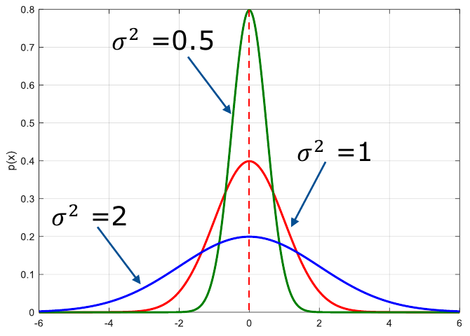
The slide labels the curves \(\sigma^2 = 0.5, 1, 2\), but the peak heights (0.8, 0.4, 0.2) only fit \(\sigma = 0.5, 1, 2\):

\[ \text{peak} = \frac{1}{\sigma\sqrt{2\pi}} \]

So read the labels as standard deviations. The lesson is the same: more spread means a lower, wider curve.

Standard normal and the z-score

A z-score tells you how many standard deviations a value is away from the mean. It lets one table (\(\Phi\)) answer every normal-distribution question.

Standard normal (\(\mu = 0\), \(\sigma = 1\)):

\[ p(x\mid 0,1) = \frac{1}{\sqrt{2\pi}} e^{-\frac{x^2}{2}} \]

The z-score:

\[ z = \frac{x - \mu}{\sigma} \]

Probability within \(k\sigma\) of the mean:

\[ P_k = \Pr[\mu - k\sigma \lt x \le \mu + k\sigma] \]

Using the standard normal:

\[ \begin{aligned} P_k &= \Pr[-k \lt z \le k] \\ &= \frac{1}{\sqrt{2\pi}}\int_{-k}^{k} e^{-\frac{z^2}{2}}dz \end{aligned} \]

In terms of the Gaussian error function erf:

\[ P_k = \operatorname{erf}(k/\sqrt2) \]

\[ P_1 \approx 68.3\% \] \[ P_2 \approx 95.4\% \] \[ P_3 \approx 99.7\% \]

Recipe (added)

Get \(\mu\) and \(\sigma\), from the question or from the sample.
\[ z = \frac{a - \mu}{\sigma} \]
“At most”: \[ P(X \le a) = \Phi(z) \]
“At least”: \[ P(X \ge a) = 1 - \Phi(z) \]
“Between”: \[ P(a \le X \le b) = \Phi(z_b) - \Phi(z_a) \]

P(X ≥ 22)

\(\bar X = 20\) and \(s_X = 2\). Assume \(X\) is normal. Use \(\Phi(1) = 0.8413\).

\[ z = \frac{22-20}{2} = 1 \]
\[ P(X\ge22) = 1 - \Phi(1) \]
\[ P(X\ge22) = 1 - 0.8413 = 0.1587 \]

For “at most”, use \(\Phi\) directly: \(P(X \le 22) = 0.8413\).

Probability of age ≥ 80

Assume age (HW1 Q3) is normal with the sample mean and standard deviation.

\[ \hat\mu = 71.45 \]
\[ \hat\sigma = \sqrt{13.8475} = 3.7212 \]
\[ z = \frac{80 - 71.45}{3.7212} = 2.30 \]
\[ P(X\ge 80) = 1 - \Phi(2.30) \]
\[ P(X\ge 80) \approx 1 - 0.9893 = 0.0107 \]

The posted HW1 key says \(P(X\ge80) = 0\). That is only true of the sample (nobody in it is 80). The question asks for the normal model, which gives about 1.1% (1.3% with \(n-1\)). Worth checking with the TA.

Multivariate normal and Mahalanobis distance

The multivariate normal is the bell curve in many dimensions. Mahalanobis distance measures how unusual a point is, allowing for the data being more spread out in some directions than others.

Joint pdf, with mean \(\boldsymbol\mu\) and covariance \(\Sigma\):

\[ p(\mathbf x \mid \boldsymbol\mu, \Sigma) = \frac{1}{\sqrt{(2\pi)^m |\Sigma|}}\; e^{-\frac12 (\mathbf x - \boldsymbol\mu)^T \Sigma^{-1}(\mathbf x-\boldsymbol\mu)} \]

Here \(|\Sigma|\) is the determinant of \(\Sigma\). The Mahalanobis distance:

\[ d_m(\mathbf x, \boldsymbol\mu) = (\mathbf x - \boldsymbol\mu)^T\Sigma^{-1}(\mathbf x - \boldsymbol\mu) \]

It generalises Euclidean distance: the distance from one observation to a set of observations, represented by their mean. If \(\Sigma = I\):

\[ d_m(\mathbf x, \boldsymbol\mu) = \|\mathbf x - \boldsymbol\mu\|^2 \]

The slide's \(d_m\) has no square root, so it is the squared Mahalanobis distance.

Mahalanobis vs Euclidean

\(\boldsymbol\mu = (0,0)\), \(\mathbf x = (2,1)\), and

\[ \Sigma = \begin{bmatrix} 4 & 0 \\ 0 & 1\end{bmatrix} \]

Squared Euclidean: \[ 2^2 + 1^2 = 5 \]
Inverse: \[ \Sigma^{-1} = \begin{bmatrix} 1/4 & 0 \\ 0 & 1\end{bmatrix} \]
Mahalanobis: \[ d_m = \frac{2^2}{4} + \frac{1^2}{1} = 2 \]

The point is exactly one standard deviation out in each direction. Mahalanobis sees that; Euclidean does not.

Part 4

The linear-algebra toolkit

Started in Lecture 3 and finished in Lecture 4. Everything in Part 5 runs on these.

Matrix multiplication you need

To multiply two matrices, multiply a row of the first by a column of the second and add the results; do that for every row–column pair.

The Quiz 2 feedback (midterm announcement 2) says many students still struggle with matrix multiplication, and every PCA step is a matrix product.

\[ (p\times q)\,(q\times r) \to (p \times r) \]

The two inner sizes must match.

Pattern 1: ZᵀZ (covariance)

For \(\mathbf Z\) of size \(n\times 2\), entry \((j,k)\) of \(\mathbf Z^T\mathbf Z\) is column \(j\) dotted with column \(k\).

\[ \mathbf Z = \begin{bmatrix} -3 & -1 \\ -1 & -3 \\ 1 & 3 \\ 3 & 1 \end{bmatrix} \]

\[ (1,1):\ 9+1+1+9 = 20 \]
\[ (1,2):\ 3+3+3+3 = 12 \]
\[ (2,2):\ 1+9+9+1 = 20 \]
\[ \mathbf Z^T\mathbf Z = \begin{bmatrix} 20 & 12 \\ 12 & 20\end{bmatrix} \]
Divide by \(n = 4\): \[ \hat\Sigma = \begin{bmatrix} 5 & 3 \\ 3 & 5\end{bmatrix} \]

Pattern 2: Σv (checking an eigenvector)

\[ \begin{bmatrix} 5 & 3 \\ 3 & 5\end{bmatrix}\begin{bmatrix} 1 \\ 1 \end{bmatrix} = \begin{bmatrix} 5+3 \\ 3+5\end{bmatrix} \]
\[ \begin{bmatrix} 8 \\ 8\end{bmatrix} = 8\begin{bmatrix} 1 \\ 1\end{bmatrix} \]

The output is the input times 8, so \((1,1)\) is an eigenvector with \(\lambda = 8\).

Pattern 3: vᵀz (projection, a dot product)

\[ \begin{bmatrix} 0.8 & 0.6 \end{bmatrix}\begin{bmatrix} -3 \\ -2 \end{bmatrix} = (0.8)(-3) + (0.6)(-2) \]
\[ = -3.6 \]

Eigen-decomposition of the covariance matrix

An eigenvector is a direction the matrix only stretches, never turns. For a covariance matrix, the eigenvectors are the main directions of the data, and each eigenvalue says how spread out the data is along its direction.

\[ \Sigma = \mathbf V \Lambda \mathbf V^T \]

\(\mathbf V\) is an \(m \times m\) orthogonal matrix whose columns are the eigenvectors:

\[ \mathbf V = [\mathbf v_1\ \mathbf v_2\ \cdots\ \mathbf v_m] \]

Each eigenvector satisfies:

\[ \Sigma\mathbf v_i = \lambda_i \mathbf v_i \]

Because \(\mathbf V\) is orthogonal:

\[ \mathbf V^T = \mathbf V^{-1} \]

\(\Lambda\) is diagonal, holding the eigenvalues:

\[ \begin{aligned} \Lambda &= \mathbf V^T\Sigma\mathbf V \\ &= \operatorname{diag}(\lambda_1, \dots, \lambda_m) \end{aligned} \]

Sign is free. \(\mathbf v\) and \(-\mathbf v\) are both correct (the Quiz 2 key says so). Flipping the sign only flips the sign of the projected coordinates.

Order differs. L3 s11 lists the small eigenvalue first; L4 s20–21 sorts largest first. PCA always uses largest first.

Solving a 2 × 2 by hand

\(\hat\Sigma\mathbf v = \lambda\mathbf v\) can be rewritten as:

\[ (\hat\Sigma - \lambda I)\mathbf v = \mathbf 0 \]

This has a non-zero solution only when:

\[ \det(\hat\Sigma - \lambda I) = 0 \]

For a 2 × 2, this is the characteristic equation:

\[ \lambda^2 - \operatorname{tr}(\hat\Sigma)\,\lambda + \det(\hat\Sigma) = 0 \]

Then, for each \(\lambda\), solve \((\hat\Sigma - \lambda I)\mathbf v = \mathbf 0\) and normalise \(\mathbf v\) to length 1.

Recipe for \(\Sigma = \begin{bmatrix} a & b \\ b & d\end{bmatrix}\)

\[ \operatorname{tr} = a + d \]
\[ \det = ad - b^2 \]
\[ \lambda = \frac{\operatorname{tr} \pm \sqrt{\operatorname{tr}^2 - 4\det}}{2} \] Sort so that \(\lambda_1 \ge \lambda_2\).
For each \(\lambda\), use one row of \((\Sigma - \lambda I)\mathbf v = 0\): \[ (a - \lambda)\,v_1 + b\,v_2 = 0 \]
Normalise: divide \(\mathbf v\) by its length. \[ \|\mathbf v\| = \sqrt{v_1^2 + v_2^2} \]
Check the sum: \[ \lambda_1 + \lambda_2 = \operatorname{tr} \]
Check the product: \[ \lambda_1\lambda_2 = \det \]

Shortcuts

Step 4 in one line (when \(b \ne 0\)):

\[ \mathbf v \propto (b,\ \lambda - a) \]

Equal diagonal \(\begin{bmatrix} a & b \\ b & a\end{bmatrix}\). Quiz 1 and notes Q6 use this. The eigenvalues are always:

\[ \lambda = a \pm b \]

For \(\lambda = a + b\), the eigenvector is:

\[ \mathbf v = \tfrac{1}{\sqrt2}(1,1) \]

For \(\lambda = a - b\), the eigenvector is:

\[ \mathbf v = \tfrac{1}{\sqrt2}(1,-1) \]

Eigenvalues and eigenvectors of the Iris Σ̂

\[ \hat\Sigma = \begin{bmatrix} 0.0904 & 0.0184 \\ 0.0184 & 0.0064\end{bmatrix} \]

Set up: \[ \det\begin{bmatrix} 0.0904 - \lambda & 0.0184 \\ 0.0184 & 0.0064 - \lambda\end{bmatrix} = 0 \]
Multiply out: \[ (0.0904-\lambda)(0.0064-\lambda) - 0.0184^2 = 0 \]
Characteristic equation: \[ \lambda^2 - 0.0968\,\lambda + 0.00024 = 0 \] (0.0968 is the trace and 0.00024 is the determinant.)
Quadratic formula: \[ \lambda = \frac{0.0968 \pm \sqrt{0.0968^2 - 4(0.00024)}}{2} \]
\[ \lambda = \frac{0.0968 \pm 0.09171}{2} \]
\[ \lambda_{\text{major}} = 0.09425 \]
\[ \lambda_{\text{minor}} = 0.00255 \]
For \(\lambda = 0.0025\): \[ \begin{bmatrix} 0.0879 & 0.0184 \\ 0.0184 & 0.0039\end{bmatrix}\mathbf v = \mathbf 0 \]
From the first row: \[ 0.0879\,v_1 = -0.0184\,v_2 \]
\[ v_2 = -4.777\,v_1 \]
Take \(v_1 = 1\): direction \((1, -4.777)\), length 4.878. \[ \mathbf v = (0.2050,\ -0.9788) \]
For \(\lambda = 0.0943\), the same steps give \(v_1 = 4.718\,v_2\). \[ \mathbf v = (0.9788,\ 0.2050) \]
Check the sum: \[ \lambda_1 + \lambda_2 = 0.0968 = \operatorname{tr}(\hat\Sigma) \]
Check the product: \[ \lambda_1\lambda_2 \approx 2.4\times10^{-4} = \det(\hat\Sigma) \]

With the shortcut, for \(\lambda_1\): \(\mathbf v \propto (0.0184,\ 0.00385)\), which normalises to \((0.979, 0.205)\). Same answer.

Eigenvalues and unit eigenvector

\[ \hat\Sigma = \begin{bmatrix} 5 & 3 \\ 3 & 5\end{bmatrix} \]

\[ (5-\lambda)^2 = 3^2 \]
\[ \lambda = 5 \pm 3 \]
\[ \lambda_1 = 8 \]
\[ \lambda_2 = 2 \]
\[ (\hat\Sigma - 8I)\mathbf v = 0 \]
First row: \[ -3v_1 + 3v_2 = 0 \]
\[ v_1 = v_2 \]
\[ \mathbf v_1 = \left(\tfrac1{\sqrt2},\ \tfrac1{\sqrt2}\right) \] Either sign is accepted.

Eigen-decomposition with a negative covariance

\[ \hat\Sigma = \begin{bmatrix} 14/3 & -7/3 \\ -7/3 & 14/3\end{bmatrix} \]

Equal diagonal, with \(a = 14/3\) and \(b = -7/3\).
\[ a - b = \tfrac{14}{3} + \tfrac{7}{3} = 7 \]
\[ a + b = \tfrac{14}{3} - \tfrac{7}{3} = \tfrac73 \]
Largest first: \[ \lambda_1 = 7 \]
Its eigenvector (from \(a - b\)): \[ \mathbf v_1 = \tfrac1{\sqrt2}(1,-1) \]
\[ \lambda_2 = \tfrac73 \]
Its eigenvector (from \(a + b\)): \[ \mathbf v_2 = \tfrac1{\sqrt2}(1,1) \]

A negative covariance puts the big direction along \((1,-1)\): when one goes up, the other goes down.

3 × 3 case (solved by computer)

HW1 Q6 asks for \(\boldsymbol\mu\), \(\Sigma\) and the eigen-decomposition of a 3-attribute data set. The posted solution uses a computer (e.g. numpy.linalg.eigh).

\[ \boldsymbol\mu = \begin{bmatrix} 1.88 \\ -0.41 \\ 2.18\end{bmatrix} \]
\[ \Sigma = \begin{bmatrix} 0.8976 & -0.2342 & 0.3846 \\ -0.2342 & 0.8889 & -0.0752 \\ 0.3846 & -0.0752 & 0.3076 \end{bmatrix} \]
Eigenvalues: 1.2512, 0.7268 and 0.1161.

Total and generalized variance

Total variance is the overall spread of the data, and it equals the sum of the eigenvalues. Generalized variance (the determinant) gets close to zero when the data is squashed almost flat.

Total variance is the trace of \(\Sigma\):

\[ \begin{aligned} \operatorname{Var}(\mathbf X) &= \sum_{i=1}^m \sigma_i^2 \\ &= \sum_{i=1}^m \lambda_i \end{aligned} \]

Why the two sums agree:

\[ \begin{aligned} \operatorname{tr}(\Sigma) &= \operatorname{tr}(V\Lambda V^{-1}) \\ &= \operatorname{tr}(\Lambda V^{-1} V) \\ &= \operatorname{tr}(\Lambda) \end{aligned} \]

Generalized variance is the determinant of \(\Sigma\):

\[ \begin{aligned} \operatorname{Gen.Var}(\mathbf X) &= |\Sigma| \\ &= \prod_{i=1}^m \lambda_i \end{aligned} \]

The eigenvalues split the total variance into pieces. The share kept by the top \(r\) directions is:

\[ \frac{\lambda_1 + \cdots + \lambda_r}{\lambda_1 + \cdots + \lambda_m} \]

PCA uses exactly this to choose \(r\) (step 5 of PCA algorithm).

Iris: total and generalized variance

\[ \Lambda = \begin{bmatrix} 0.0025 & 0 \\ 0 & 0.0943\end{bmatrix} \]
\[ \mathbf V = \begin{bmatrix} 0.2050 & -0.9788 \\ -0.9788 & -0.2050\end{bmatrix} \]
Sum of the diagonal: \[ 0.0064 + 0.0904 = 0.0968 \]
Sum of the eigenvalues: \[ 0.09425 + 0.00255 = 0.0968 \]
Determinant: \[ |\hat\Sigma| = (0.0904)(0.0064) - 0.0184^2 \]
\[ |\hat\Sigma| = 2.4\times10^{-4} \]

Share on the top direction: \(0.09425 / 0.0968 = 97.4\%\). The cloud is almost a line.

Share of variance on the first PC

The eigenvalues are 8 and 2.

\[ \frac{\lambda_1}{\lambda_1 + \lambda_2} = \frac{8}{10} \]
\[ = 0.8 \ (80\%) \]

Change of basis and projection

Projecting a point onto a direction means finding its shadow on that line. The shadow's coordinate is a dot product, and the part you lose sits at a right angle to the line.

Added diagram, after L4 s11 and s15: the projection x̃ and the error ε meet at a right angle.

Coordinates in a new basis

Standard basis vectors:

\[ \begin{aligned} \mathbf e_1^T &= [1,0,\dots,0] \\ &\ \ \vdots \\ \mathbf e_m^T &= [0,\dots,0,1] \end{aligned} \]

Any point is a weighted sum of them:

\[ \mathbf x = x_1\mathbf e_1 + \cdots + x_m\mathbf e_m \]

In a new coordinate system \(\mathbf v_i\), the component of \(\mathbf x\) along \(\mathbf v_i\) is its projection:

\[ y_i = \mathbf v_i^T\mathbf x \]

If the \(\mathbf v_i\) are orthonormal (length 1, at right angles), \(\mathbf x\) is rebuilt from its new coordinates:

\[ \begin{aligned} \mathbf x &= y_1\mathbf v_1 + \cdots + y_m\mathbf v_m \\ &= V\mathbf y \end{aligned} \]

Multiply both sides by \(V^T\), and use \(V^TV = I\):

\[ \mathbf y = V^T\mathbf x \]

With the \(\mathbf v_i\) sorted by importance, keep only the first \(r\) terms:

\[ \begin{aligned} \tilde{\mathbf x}_r &= y_1\mathbf v_1 + \cdots + y_r\mathbf v_r \\ &= V_r\mathbf y_r \end{aligned} \]

The rest is close to a null vector:

\[ \mathbf x - \tilde{\mathbf x}_r = y_{r+1}\mathbf v_{r+1} + \cdots + y_m\mathbf v_m \approx \mathbf 0 \]

Lecture 1's projection was \(\operatorname{proj}_{\mathbf v}\mathbf u = \frac{\mathbf u\cdot\mathbf v}{\|\mathbf v\|^2}\mathbf v\). When \(\|\mathbf v\| = 1\), this becomes \(y\,\mathbf v\) with \(y = \mathbf v^T\mathbf u\): the same thing.

Coordinates of x = (10, 8)

\[ \mathbf x = \begin{bmatrix} 10 \\ 8\end{bmatrix} \] \[ \mathbf v_1 = \begin{bmatrix} 0.8 \\ 0.6\end{bmatrix} \] \[ \mathbf v_2 = \begin{bmatrix} -0.6 \\ 0.8\end{bmatrix} \]

\[ \mathbf y = \begin{bmatrix} 0.8 & 0.6 \\ -0.6 & 0.8\end{bmatrix}\begin{bmatrix} 10 \\ 8\end{bmatrix} \]
\[ \mathbf y = \begin{bmatrix} 12.8 \\ 0.4\end{bmatrix} \]
Rebuild: \[ \mathbf x = 12.8\begin{bmatrix} 0.8 \\ 0.6\end{bmatrix} + 0.4\begin{bmatrix} -0.6 \\ 0.8\end{bmatrix} = \begin{bmatrix} 10 \\ 8\end{bmatrix} \]
Keep only \(\mathbf v_1\): \[ \tilde{\mathbf x}_1 = 12.8\,\mathbf v_1 = \begin{bmatrix} 10.24 \\ 7.68\end{bmatrix} \]
Error: \[ y_2\mathbf v_2 = \begin{bmatrix} -0.24 \\ 0.32\end{bmatrix} \]
Check the right angle (added): \[ (-0.24)(10.24) + (0.32)(7.68) = 0 \]

Projection onto a subspace

\(\mathbf v_1, \dots, \mathbf v_r\) span an \(r\)-dimensional subspace. The projection onto it:

\[ \begin{aligned} \tilde{\mathbf x}_r &= V_rV_r^T\mathbf x \\ &= P_r\mathbf x \end{aligned} \]

The projection matrix:

\[ \begin{aligned} P_r &= V_rV_r^T \\ &= \sum_{i=1}^r \mathbf v_i\mathbf v_i^T \end{aligned} \]

Its properties:

\[ P_r^T = P_r \] \[ P_r^2 = P_r \]

The error is the projection onto the remaining directions:

\[ \begin{aligned} \boldsymbol\epsilon &= \mathbf x - \tilde{\mathbf x} \\ &= (I - P_r)\mathbf x \end{aligned} \]

The error and the projection are at right angles:

\[ \boldsymbol\epsilon^T\tilde{\mathbf x} = 0 \]

\(P_r\) is the “drop it onto the subspace” machine. \(P_r^2 = P_r\) because dropping something that is already there changes nothing.

Decorrelation (promised in L3's outline)

Lecture 3's outline lists “Linear transformation of RV: decorrelation”, but no slide covers it. Take new coordinates along the eigenvectors of \(\Sigma\):

\[ \mathbf y = V^T(\mathbf x - \boldsymbol\mu) \]

Their covariance is diagonal (L3 s10):

\[ \begin{aligned} \operatorname{Cov}(\mathbf y) &= V^T\Sigma V \\ &= \Lambda \end{aligned} \]

So in eigenvector coordinates, every pair of new variables has covariance 0: they are decorrelated.

Projecting u onto v

\(\mathbf u = (3,4)\) and \(\mathbf v = (3,0)\).

\[ \operatorname{proj}_{\mathbf v}\mathbf u = \frac{\mathbf u\cdot\mathbf v}{\|\mathbf v\|^2}\,\mathbf v \]
\[ = \frac{9}{9}\begin{bmatrix} 3 \\ 0\end{bmatrix} \]
\[ = \begin{bmatrix} 3 \\ 0\end{bmatrix} \]

Projecting V₁ onto V₂

\(V_1 = [1\ 2\ 3\ 4\ 5]^T\) and \(V_2 = [5\ {-4}\ 3\ {-2}\ 1]^T\).

\[ \frac{V_1^TV_2}{V_2^TV_2} = \frac{3}{55} = 0.0545 \]
\[ \operatorname{proj}_{V_2}V_1 = 0.0545\,V_2 \]
\[ = [0.2727\ \ {-0.2182}\ \ 0.1636\ \ {-0.1091}\ \ 0.0545]^T \]

Part 5

Principal Component Analysis

Why PCA?

PCA shrinks data with many columns into a few new columns while keeping most of the information. It works because real features are usually related, so a few directions hold most of the spread.

Real data is high-dimensional: a 28 × 28 image is 784 numbers, a BERT sentence embedding has 768, and a gene-expression profile can have tens of thousands.
That is costly: storage and computation grow with \(m\); k-NN and k-means slow down and get worse (the curse of dimensionality); and you cannot plot more than 2–3 dimensions.
The key fact PCA uses: features are rarely independent, so a handful of directions capture most of the variation.
Pipeline: raw features (\(m\) dims) → keep the top \(r\) eigenvectors → compressed data (\(r \ll m\)) → plots, search, classifiers.
Uses: compression (faces as a mix of a few “eigenfaces”), visualisation (plot the top 2–3 PCs), and preprocessing (decorrelate and denoise before a classifier).

The best direction is the top eigenvector

The first principal component is the direction where the data is most spread out. It is the eigenvector with the largest eigenvalue, and that eigenvalue equals the spread along it.

Find the unit direction \(\mathbf v\) that maximises the variance of the data projected onto it. Assume zero mean and \(\|\mathbf v\| = 1\).

The projection of a point onto \(\mathbf v\):

\[ y = \mathbf v^T\mathbf x \] \[ \tilde{\mathbf x} = (\mathbf v^T\mathbf x)\,\mathbf v \]

Since the mean is zero, \(E[y] = 0\). The variance along \(\mathbf v\):

\[ \begin{aligned} \operatorname{Var}(y) &= E[y^2] \\ &= E[\mathbf v^T\mathbf x\mathbf x^T\mathbf v] \\ &= \mathbf v^T\Sigma\mathbf v \end{aligned} \]

If \(\mathbf v\) is an eigenvector, \(\Sigma\mathbf v = \lambda\mathbf v\), so:

\[ \begin{aligned} \operatorname{Var}(y) &= \lambda\,\mathbf v^T\mathbf v \\ &= \lambda \end{aligned} \]

Each eigenvalue is the variance along its eigenvector.
The largest eigenvalue gives the largest variance. Its eigenvector is the first principal component.
The eigenvector of the smallest eigenvalue is the first minor component.

Real data rarely has zero mean, so subtract the mean first:

\[ y = \mathbf v^T(\mathbf x - \boldsymbol\mu) \]

Quiz 2 feedback: many students skipped this check. If the mean is already \(\mathbf 0\), say so in your answer.

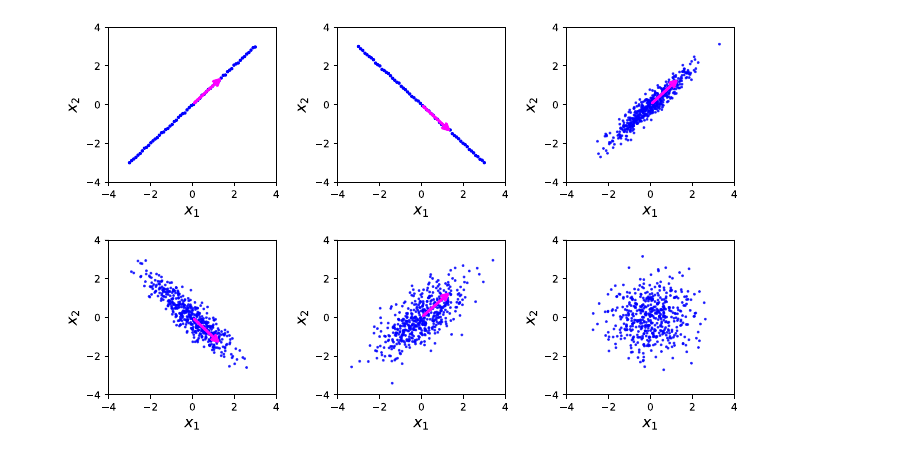
Six scatter plots of 2-D data with the first principal component drawn as a magenta arrow — L4 s17: the magenta arrow is the first principal component. In the round cloud (bottom right), no direction stands out, so PCA has nothing to compress.

Project onto u₁ and recover λ₁

Problem reconstructed from the posted solution sheet. Same data as HW2 Q2.

Data: \(\mathbf x_1 = (-3,-2)\), \(\mathbf x_2 = (1,0)\), \(\mathbf x_3 = (2,2)\). First principal direction (rounded): \(\mathbf u_1 = (0.8, 0.6)\).

(a) Find \(a_i = \mathbf u_1^T(\mathbf x_i - \boldsymbol\mu)\). (b) Use (a) to find \(\lambda_1\).

Check the mean: \[ \boldsymbol\mu = \tfrac13(-3+1+2,\ -2+0+2) = (0,0) \] Already centered.
\[ a_1 = 0.8(-3) + 0.6(-2) = -3.6 \]
\[ a_2 = 0.8(1) + 0.6(0) = 0.8 \]
\[ a_3 = 0.8(2) + 0.6(2) = 2.8 \]
The eigenvalue is the variance of the projections: \[ \lambda_1 = \frac1n\sum a_i^2 \]
\[ \lambda_1 = \frac{12.96 + 0.64 + 7.84}{3} \]
\[ \lambda_1 = \frac{21.44}{3} = 7.147 \]

Exact value from \(\det(\Sigma - \lambda I) = 0\): \(\lambda_1 = (11 + \sqrt{109})/3 = 7.1468\).

Two views of “best”, and more than one component

The line where the data is most spread out is also the line the points sit closest to, so both ideas of “best” give the same answer. For more components, take the next eigenvectors in order.

View 1, maximum variance:

\[ \max_{\mathbf v}\ \mathbf v^T\Sigma\mathbf v \quad\text{subject to } \|\mathbf v\|^2 = 1 \]

View 2, minimum mean squared error between \(\mathbf x\) and its projection:

\[ \min_{\mathbf v}\ E[\|\mathbf x - \tilde{\mathbf x}\|^2] \quad\text{subject to } \tilde{\mathbf x} = (\mathbf v^T\mathbf x)\mathbf v,\ \|\mathbf v\|^2 = 1 \]

After some algebra, view 2 becomes:

\[ \min_{\mathbf v}\ E[\mathbf x^T\mathbf x] - \mathbf v^T E[\mathbf x\mathbf x^T]\,\mathbf v \]

\(E[\mathbf x^T\mathbf x]\) is the total variance (a constant) and \(E[\mathbf x\mathbf x^T] = \Sigma\). So view 2 is the same as view 1.

More components: given \(\mathbf v_1, \dots, \mathbf v_{r-1}\), find the best direction at right angles to all of them:

\[ \max_{\mathbf v}\ \mathbf v^T\Sigma\mathbf v \quad\text{s.t. } \|\mathbf v\|^2 = 1,\ \ \mathbf v^T\mathbf v_i = 0 \]

The answer is the \(r\)-th eigenvector. So the best \(r\)-dimensional approximation projects onto the first \(r\) eigenvectors.

The kept part and the lost part are at right angles, so Pythagoras applies:

\[ \|\mathbf x\|^2 = y^2 + \|\boldsymbol\epsilon\|^2 \]

The left side is fixed, so making the kept part (\(y^2\)) bigger makes the lost part smaller.

The mean squared reconstruction error equals the sum of the eigenvalues you dropped:

\[ \frac1n\sum_i \|\mathbf x_i - \tilde{\mathbf x}_i\|^2 = \lambda_{r+1} + \cdots + \lambda_m \]

Checked with numpy: Iris (\(r=1\)) gives 0.00255 = \(\lambda_2\); HW2 Q2 gives 0.1866 = \(\lambda_2\).

The PCA algorithm

Center the data, build the covariance matrix, take its top eigenvectors, and project the data onto them.

Input: the \(n\times m\) data matrix \(X\) (rows = samples) and a target \(0 \lt \alpha \lt 1\).

Mean: \[ \boldsymbol\mu = \frac1n\sum_{i=1}^n\mathbf x_i \]
Center: \[ Z = X - \mathbf 1\boldsymbol\mu^T \]
Covariance (\(m\times m\)): \[ \Sigma = \frac1n Z^TZ \]
Eigen-decomposition, sorted \(\lambda_1 \ge \cdots \ge \lambda_m\): \[ \Sigma = V\Lambda V^T \]
Choose \(r\): the smallest integer with \[ \alpha \le \frac{\sum_{i=1}^r\lambda_i}{\sum_{i=1}^m\lambda_i} \]
Keep the first \(r\) eigenvectors: \[ V_r = [\mathbf v_1, \dots, \mathbf v_r] \]
New coordinates of each sample: \[ \mathbf y_i = V_r^T(\mathbf x_i - \boldsymbol\mu) \]
Rebuilt sample: \[ \tilde{\mathbf x}_i = P_r(\mathbf x_i - \boldsymbol\mu) + \boldsymbol\mu \] where \(P_r = V_rV_r^T\).

Sizes: \(V_r\) is \(m\times r\), \(\mathbf y_i\) is \(r\times1\), \(\tilde{\mathbf x}_i\) and \(\boldsymbol\mu\) are \(m\times1\), and \(P_r\) is \(m\times m\).

1–2: Moves the cloud so it is centred at the origin.
3: The table of spreads and co-movements.
4: The main directions and how much spread each one holds.
5: \(\alpha\) answers “how much of the variance must I keep?”, e.g. 0.95.
6–7: The new, shorter coordinates (the “scores”).
8: The point rebuilt from those scores, back in original units.

Check whether the data is already centered, and say so.
Show every step. A bare final answer gets no credit.
Say which eigenvalue is largest, and that this makes its eigenvector the first PC.
Either sign of an eigenvector is fine. Keep the same sign throughout.
If stuck, write the formula anyway: partial credit is available.

Full PCA on the 5 Iris flowers

Mean (from L3 s9): \[ \boldsymbol\mu = (4.54,\ 1.44) \]
Centered data: \[ Z^T = \begin{bmatrix} 0.16 & -0.04 & 0.36 & -0.54 & 0.06 \\ -0.04 & 0.06 & 0.06 & -0.14 & 0.06\end{bmatrix} \]
Covariance: \[ \hat\Sigma = \begin{bmatrix} 0.0904 & 0.0184 \\ 0.0184 & 0.0064\end{bmatrix} \]
Characteristic equation: \[ \lambda^2 - 0.0968\,\lambda + 0.00024 = 0 \]
\[ \lambda = \frac{0.0968 \pm 0.09171}{2} \]
\[ \lambda_1 = 0.09425 \]
\[ \lambda_2 = 0.00255 \]
First eigenvector (tracks petal length, tilted toward petal width): \[ \mathbf v_1 = (0.9788,\ 0.2050) \]
Second eigenvector: \[ \mathbf v_2 = (0.2050,\ -0.9788) \]
Variance kept with \(r = 1\): \[ \frac{\lambda_1}{\lambda_1 + \lambda_2} \approx 97.4\% \] With \(\alpha = 0.95\), \(r = 1\) is enough.

Project each centered point: \[ y_i = \mathbf v_1^T\mathbf z_i \]

i	z_i	y_i
1	(0.16, −0.04)	0.148
2	(−0.04, 0.06)	−0.027
3	(0.36, 0.06)	0.365
4	(−0.54, −0.14)	−0.557
5	(0.06, 0.06)	0.071

Check: \[ \operatorname{Var}(y) = \frac15\sum y_i^2 = 0.0943 \approx \lambda_1 \]

\[ \tilde{\mathbf x}_1 = y_1\mathbf v_1 + \boldsymbol\mu \] \[ \tilde{\mathbf x}_1 = 0.148\begin{bmatrix} 0.9788 \\ 0.2050\end{bmatrix} + \begin{bmatrix} 4.54 \\ 1.44\end{bmatrix} \] \[ \tilde{\mathbf x}_1 = \begin{bmatrix} 4.685 \\ 1.470\end{bmatrix} \]

The actual flower is \((4.7, 1.4)\): one number instead of two, and still close.

Full PCA on six points

Points \((2,3), (4,5), (3,4), (5,7), (6,7), (7,8)\). Use \(1/n\). (a) mean; (b) centered data; (c) \(\Sigma\); (d) eigenvalues and eigenvectors; (e) the principal component and its share of variance; (f) project the centered data onto it.

(a) \[ \boldsymbol\mu = \left(\tfrac{27}{6},\ \tfrac{34}{6}\right) = (4.5,\ 5.6667) \]
(b) Rows of \(Z\): \((-2.5, -2.667)\), \((-0.5, -0.667)\), \((-1.5, -1.667)\), \((0.5, 1.333)\), \((1.5, 1.333)\), \((2.5, 2.333)\).
(c) Sums of products: 17.5, 18 and 19.333. Divide by 6: \[ \Sigma = \begin{bmatrix} 2.9167 & 3.0000 \\ 3.0000 & 3.2222\end{bmatrix} \]
(d) \[ \operatorname{tr} = 6.1389 \]
\[ \det = 0.3981 \]
\[ \lambda = \frac{6.1389 \pm \sqrt{37.686 - 1.593}}{2} \]
\[ \lambda = \frac{6.1389 \pm 6.0078}{2} \]
\[ \lambda_1 = 6.0733 \]
\[ \lambda_2 = 0.0656 \]
Shortcut: \[ \mathbf v_1 \propto (3,\ 6.0733 - 2.9167) = (3,\ 3.1566) \]
Normalise: \[ \mathbf v_1 = (0.6889,\ 0.7249) \]
At right angles: \[ \mathbf v_2 = (-0.7249,\ 0.6889) \]
(e) \(\mathbf v_1\) is the PC (largest eigenvalue). \[ \frac{6.0733}{6.1389} = 98.9\% \]
(f) \[ y_i = \mathbf v_1^T\mathbf z_i \]
\[ \mathbf y = (-3.655,\ -0.828,\ -2.241,\ 1.311,\ 2.000,\ 3.414) \]
Check: \[ \tfrac16\sum y_i^2 = 6.073 = \lambda_1 \]

The posted HW2 key (from the 2025 run) lists scores 3.55, 6.38, 4.97, …. Those come from the raw, uncentered points, and they are off from the centered scores by a constant:

\[ \mathbf v_1^T\boldsymbol\mu = 7.208 \]

This year's question and L4 s20 both use \(\mathbf y = V^T(\mathbf x - \boldsymbol\mu)\), so use the centered values.

PCA, projection and reconstruction error

Three points given as the columns of the matrix below. Use \(1/n\). (a) covariance matrix; (b) first PC; (c) 1-D coordinates and their variance; (d) rebuild in 2-D and find the mean squared error.

\[ \begin{bmatrix} -3 & 1 & 2 \\ -2 & 0 & 2\end{bmatrix} \]

Rows = samples: \((-3,-2)\), \((1,0)\), \((2,2)\). The mean is \((0,0)\), so the data is already centered.
(a) \[ \Sigma = \frac13\begin{bmatrix} 14 & 10 \\ 10 & 8\end{bmatrix} \]
\[ \Sigma = \begin{bmatrix} 4.667 & 3.333 \\ 3.333 & 2.667\end{bmatrix} \]
(b) \[ \operatorname{tr} = \tfrac{22}{3} \]
\[ \det = \tfrac43 \]
\[ \lambda = \frac{11 \pm \sqrt{109}}{3} \]
\[ \lambda_1 = 7.1468 \]
\[ \lambda_2 = 0.1866 \]
\[ \mathbf v_1 \propto (3.333,\ 2.480) \]
\[ \mathbf v_1 = (0.8023,\ 0.5969) \]
(c) \[ \mathbf y = (-3.6007,\ 0.8023,\ 2.7984) \]
\[ \operatorname{Var}(y) = \tfrac13\sum y_i^2 = 7.147 = \lambda_1 \]
(d) Rebuild each point: \[ \tilde{\mathbf x}_i = y_i\,\mathbf v_1 \] This gives \((-2.889, -2.149)\), \((0.644, 0.479)\) and \((2.245, 1.670)\).
Errors \(\mathbf x_i - \tilde{\mathbf x}_i\): \((-0.111, 0.149)\), \((0.356, -0.479)\) and \((-0.245, 0.330)\).
Squared lengths: 0.0347, 0.3563 and 0.1687. \[ \text{sum} = 0.5597 \]
\[ \text{MSE} = \frac{0.5597}{3} = 0.1866 = \lambda_2 \]

The 2025 key reports the sum (0.5597) and uses \(n-1\) in part (a). This year's question says \(1/n\).

Which eigenvector is the first principal direction?

From notes Q6: \(\lambda_1 = 7\) with \(\mathbf v_1 = \tfrac1{\sqrt2}(1,-1)\), and \(\lambda_2 = 7/3\) with \(\mathbf v_2 = \tfrac1{\sqrt2}(1,1)\).

\(\mathbf v_1\), because its eigenvalue is the largest, so it captures the most variance:

\[ \frac{7}{7 + 7/3} = 75\% \]

Part 6

Exam toolkit

The midterm gives you the formulas. The skill being tested is picking the right one.

Which formula, when

The question asks for…	Use	Card
spread of one variable	\(\hat\sigma^2 = \frac1n\sum(x_i - \hat\mu)^2\)	Mean
how two variables move together	\(\hat\sigma_{12} = \frac1n\sum(x_{1i}-\hat\mu_1)(x_{2i}-\hat\mu_2)\)	Covariance
all spreads at once	\(\hat\Sigma = \frac1n Z^TZ\)	Cov. matrix
strength of a straight-line relationship	\(\rho = \sigma_{12}/(\sigma_1\sigma_2)\)	Correlation
a probability under a normal model	\(z = (x-\mu)/\sigma\), then the \(\Phi\) table	z-score
distance that allows for spread	\((\mathbf x-\boldsymbol\mu)^T\Sigma^{-1}(\mathbf x-\boldsymbol\mu)\)	Mahalanobis
eigenvalues	\(\det(\Sigma - \lambda I) = 0\)	By hand
eigenvalues of a 2 × 2	\(\lambda^2 - \operatorname{tr}\,\lambda + \det = 0\)	By hand
eigenvector for a given \(\lambda\)	\((\Sigma - \lambda I)\mathbf v = 0\), then normalise	By hand
total variance	\(\operatorname{tr}\Sigma = \sum\lambda_i\)	Total var.
generalized variance	\(\|\Sigma\| = \prod\lambda_i\)	Total var.
share of variance / how many components	\(\sum_{i\le r}\lambda_i \,/\, \sum_i\lambda_i \ge \alpha\)	Algorithm
coordinates on the PCs (“project the data”)	\(\mathbf y_i = V_r^T(\mathbf x_i - \boldsymbol\mu)\)	Algorithm
variance of the projected data	\(\lambda\) (the mean of \(y_i^2\))	Best direction
rebuild a point in original units	\(\tilde{\mathbf x}_i = V_r\mathbf y_i + \boldsymbol\mu\)	Algorithm
reconstruction error	mean \(\\|\mathbf x_i - \tilde{\mathbf x}_i\\|^2\) = sum of dropped \(\lambda\)	Two views