From kernels to kernel PCA
Lecture 5 (High-Dimensional Data and Kernel Methods) and Lecture 6 (Kernel PCA), rebuilt as one storyline. Lecture 6 restates most of Lecture 5 with more examples, so each idea appears once here with both sources.
How to read this page. Ordered by concept, not by slide. Lecture 5 introduces kernels; Lecture 6 recaps them (its slides 2–4) and then builds kernel PCA on top. Every card says which slides it came from, what it needs, and what uses it. This page assumes the Lectures 3–4 page: covariance, eigen-decomposition, projection and the PCA algorithm.
Teal = explanation added by Claude, not on the slides. Amber = watch out. Dropdowns hide worked examples, practice questions, and their answers.
The road to kernel PCA
The “curse of dimensionality” (Part 1) is a side branch: it motivates kernels and explains HW1 Q7, but kernel PCA does not use its formulas.
Lecture map: which slides each card covers
Lecture 5 prints two slides as “6”. The second one (Nonlinear PCA) is called s6b here.
Part 1
Why linear PCA is not enough
Side branch. Read it once for the ideas; the formulas are not used later.
Data in high dimensions: hypercube and hyperball
With many attributes, the data lives in a huge box, but the points fill only a tiny part of it. Distances and angles stop behaving the way they do in 2-D.
- \(m\)
- number of attributes = the dimension
- \(L\)
- half the side of the box: the biggest radius over all attributes
- \(r\)
- radius of the ball: the length of the longest point
- ball vs sphere
- the ball is the solid; the sphere is only its skin
The ball inside the cube shrinks
In 2-D a circle fills most of its square. As dimensions grow, the ball fills almost none of the cube, so almost all the room is in the corners.
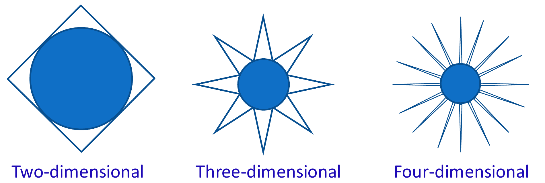
A random unit vector in \(\mathbb R^{30}\) almost never lands near one chosen direction, because the sphere's surface is spread over a huge number of “corners”. That is why 100,000 random tries still lose to the eigenvector, which the eigen-decomposition finds directly.
Diagonals become orthogonal to every axis
In high dimensions the diagonal of the cube is almost at right angles to every axis. A cluster sitting near a diagonal collapses to the origin when you project it on any axis.
How fast the angle grows
- \(m = 2\): \[ \cos\theta = \frac{1}{\sqrt 2} = 0.707 \] so \(\theta = 45^\circ\).
- \(m = 30\) (HW1 Q7): \[ \cos\theta = \frac{1}{\sqrt{30}} = 0.183 \] so \(\theta = 79.5^\circ\).
- \(m = 784\) (one MNIST image): \[ \cos\theta = \frac{1}{\sqrt{784}} = 0.036 \] so \(\theta = 88^\circ\).
Linear PCA cannot see a curve
PCA only rotates the axes, so it cannot straighten a curved pattern. If you first transform the data with a non-linear function, PCA works again.
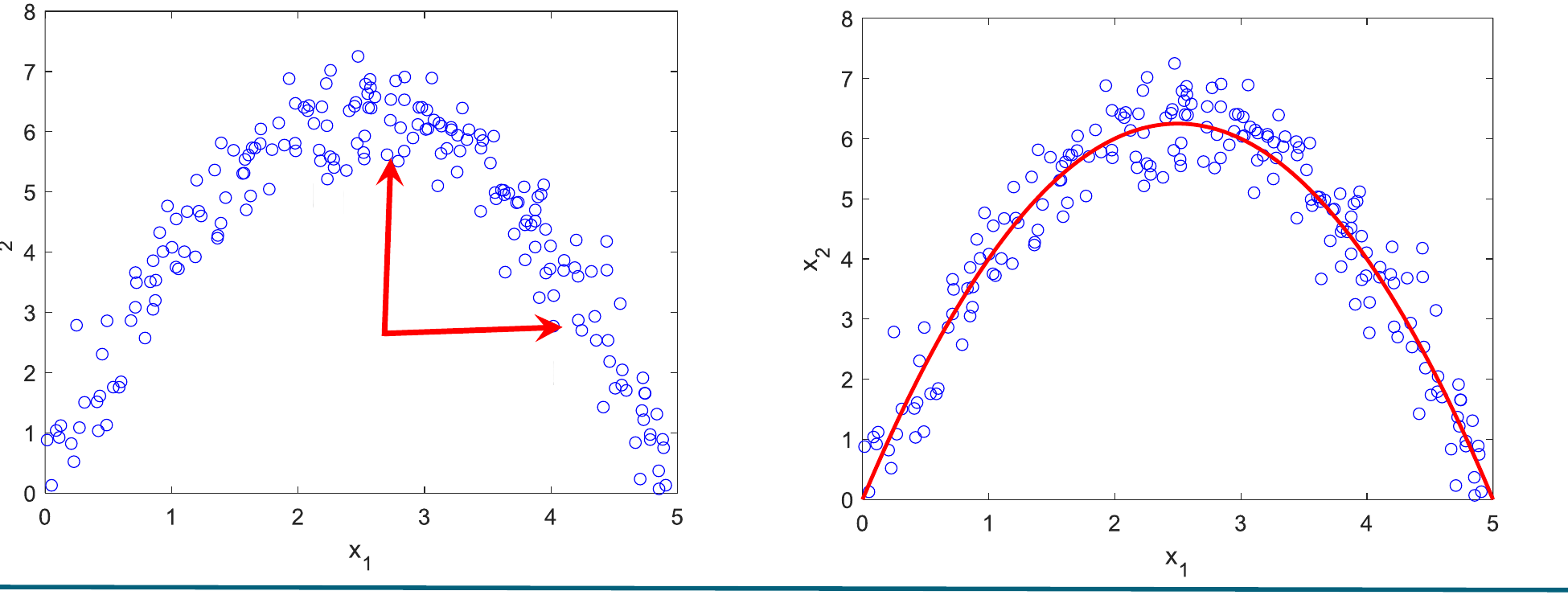
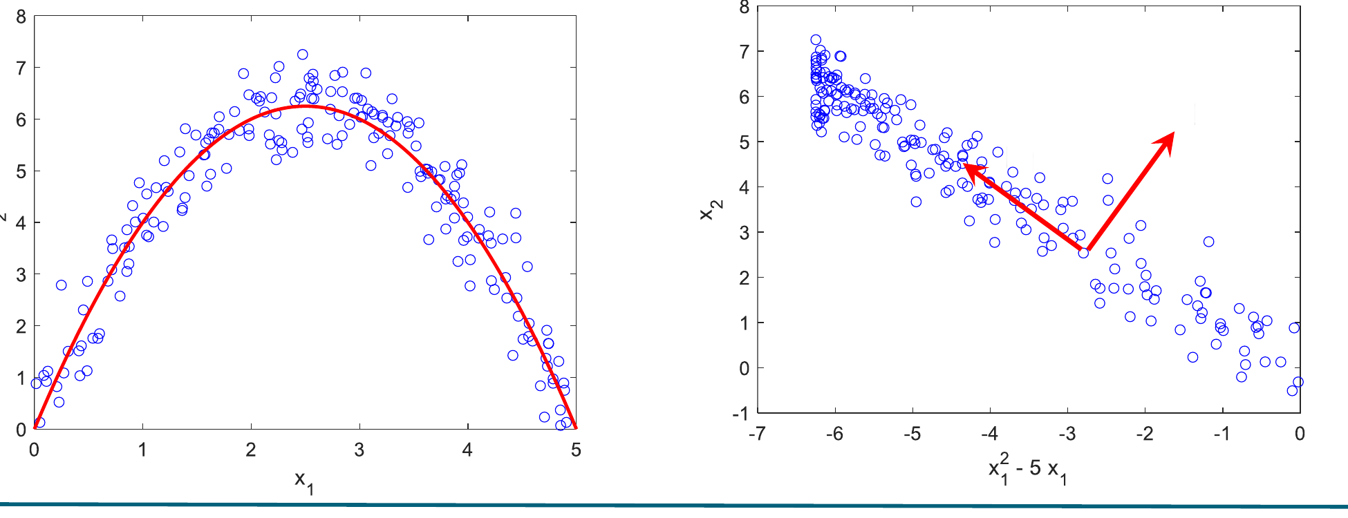
Before the transform the two eigenvalues are similar (3.41 and 1.73), so no single direction explains the data. After it, one eigenvalue dominates (7.04 vs 0.11): one direction is enough. The transform \(\phi\) is the first example of a feature map, the next card.
Part 2
Kernels: inner products in a bigger space
Feature map and the kernel trick
A feature map sends each point to a longer vector made of its squares and products. The kernel trick is that the dot product of two mapped vectors can be computed from the original dot product, without ever writing the long vectors.
- \(\phi\)
- the feature map: input vector in, longer feature vector out
- \(\phi(\mathbf x)\)
- the point in feature space (we usually never compute it)
- \(K(\mathbf x, \mathbf y)\)
- the kernel: a number, equal to \(\phi(\mathbf x)^T \phi(\mathbf y)\)
- \(\sqrt 2\)
- makes the cross term come out as \(2 x_1 x_2 y_1 y_2\) when squared
Expand the square of a two-term sum:
\[ (x_1 y_1 + x_2 y_2)^2 = x_1^2 y_1^2 + 2\, x_1 y_1 x_2 y_2 + x_2^2 y_2^2 \]The middle term must come from one coordinate of \(\phi\). Writing that coordinate as \(\sqrt 2\, x_1 x_2\) gives \((\sqrt 2\, x_1 x_2)(\sqrt 2\, y_1 y_2) = 2 x_1 x_2 y_1 y_2\). With \(m\) inputs there is one such coordinate per pair, so \(\phi\) has \(m\) squares plus \(\binom m2\) cross terms: 3 coordinates for \(m = 2\), 6 for \(m = 3\).
Map one vector
- \[ \mathbf x = (-0.5,\ \sqrt 2)^T \]
- \[ x_1^2 = 0.25 \]
- \[ x_2^2 = 2 \]
- \[ \sqrt 2\, x_1 x_2 = \sqrt 2 \times (-0.5) \times \sqrt 2 = -1 \]
- \[ \phi(\mathbf x) = (0.25,\ 2,\ -1)^T \]
Both routes give 25
\(\mathbf x = [2\ \ 1]^T\), \(\mathbf y = [1\ \ 3]^T\).
- Kernel route: \[ \mathbf x^T \mathbf y = 2 \times 1 + 1 \times 3 = 5 \]
- \[ K(\mathbf x, \mathbf y) = 5^2 = 25 \]
- Feature route: \[ \phi(\mathbf x) = (4,\ 1,\ 2\sqrt 2)^T \]
- \[ \phi(\mathbf y) = (1,\ 9,\ 3\sqrt 2)^T \]
- \[ \phi(\mathbf x)^T \phi(\mathbf y) = 4 + 9 + 12 = 25 \] Same answer, and the kernel route never needed \(\phi\).
Six-dimensional feature vectors
\(\mathbf x = (-1, 0, 1)^T\), \(\mathbf y = (1, -2, -1)^T\), kernel \(K(\mathbf x, \mathbf y) = (\mathbf x^T \mathbf y)^2\). Find \(\phi(\mathbf x)\), \(\phi(\mathbf y)\), and check the kernel value.
- \[ \mathbf x^T \mathbf y = -1 + 0 - 1 = -2 \]
- \[ K(\mathbf x, \mathbf y) = (-2)^2 = 4 \]
- Order of coordinates: \(x_1^2, x_2^2, x_3^2, \sqrt2 x_1 x_2, \sqrt2 x_1 x_3, \sqrt2 x_2 x_3\). \[ \phi(\mathbf x) = (1,\ 0,\ 1,\ 0,\ -\sqrt 2,\ 0)^T \]
- \[ \phi(\mathbf y) = (1,\ 4,\ 1,\ -2\sqrt 2,\ -\sqrt 2,\ 2\sqrt 2)^T \]
- \[ \phi(\mathbf x)^T \phi(\mathbf y) = 1 + 0 + 1 + 0 + 2 + 0 = 4 \] It matches the kernel value.
Kernel functions: polynomial and RBF
A kernel is any function of two points that equals a dot product in some feature space. The two you need are the polynomial kernel and the Gaussian (RBF) kernel.
- \(p\)
- degree of the polynomial (1 = linear, 2 = quadratic)
- \(c\)
- constant added before raising to the power; \(c = 0\) gives the homogeneous kernel \((\mathbf x^T \mathbf y)^p\)
- \(\gamma\)
- width parameter of the RBF kernel; bigger \(\gamma\) makes similarity fall faster with distance
- \(\|\mathbf x - \mathbf y\|^2\)
- squared Euclidean distance: sum of squared coordinate differences
Every point has feature-space length 1, and far-apart points have a kernel value near 0. The feature space of the RBF kernel is infinite-dimensional, so \(\phi\) can never be written out: everything must go through \(K\).
HW2 Q3 and Quiz 2 use \((\mathbf x^T \mathbf y)^2\), with no constant. L5 s12–14 and L6 Example 3 use \((1 + \mathbf x^T \mathbf y)^2\). Read the question before squaring.
Same two points, three kernels
\(\mathbf x = (2, 3)^T\), \(\mathbf y = (-1, 1)^T\). First \(\mathbf x^T \mathbf y = -2 + 3 = 1\) and \(\|\mathbf x - \mathbf y\|^2 = 3^2 + 2^2 = 13\).
- Linear, \(c = 0\): \[ K = 1 \]
- Quadratic, \(c = 1\): \[ K = (1 + 1)^2 = 4 \]
- Homogeneous quadratic, \(c = 0\): \[ K = 1^2 = 1 \]
- RBF, \(\gamma = 0.1\): \[ K = e^{-0.1 \times 13} = e^{-1.3} = 0.2725 \]
The kernel matrix and its properties
The kernel matrix stores the kernel value for every pair of points. It is a table of similarities, and it is all that kernel methods ever look at.
Recipe: kernel matrix by hand
- Write the points as columns of \(X\) and compute the Gram matrix \(X^T X\) (every pairwise dot product). For \(n\) points that is \(n(n+1)/2\) distinct dot products.
- Polynomial kernel: apply \((c + \cdot)^p\) to every entry. The slide writes this with the entry-wise (Hadamard) product \(\circ\): \[ \mathbf K_2 = (1 + X^T X) \circ (1 + X^T X) \]
- RBF kernel: first build the squared-distance matrix \(D = [\delta_{ij}]\) with \(\delta_{ij} = \|\mathbf x_i - \mathbf x_j\|^2\), then \[ \mathbf K_{RBF} = [e^{-\gamma \delta_{ij}}] \]
- Check: symmetric, diagonal \(\ge 0\) (RBF diagonal is exactly 1).
\(\|\mathbf x_i - \mathbf x_j\|^2 = \mathbf x_i^T \mathbf x_i + \mathbf x_j^T \mathbf x_j - 2\, \mathbf x_i^T \mathbf x_j\). So the Gram matrix also gives you \(D\): diagonal entry plus diagonal entry minus twice the off-diagonal entry.
Quadratic (c = 1) and RBF (γ = 0.1) kernel matrices for three points
Points as columns:
\[ X = \begin{bmatrix} -1 & 1 & 2 \\ 0 & -1 & 1 \\ 1 & 0 & -2 \end{bmatrix} \]- \[ X^T X = \begin{bmatrix} 2 & -1 & -4 \\ -1 & 2 & 1 \\ -4 & 1 & 9 \end{bmatrix} \]
- Add 1 to every entry, then square every entry: \[ \mathbf K_2 = \begin{bmatrix} 9 & 0 & 9 \\ 0 & 9 & 4 \\ 9 & 4 & 100 \end{bmatrix} \]
- Squared distances, e.g. \(\delta_{12} = 2 + 2 - 2(-1) = 6\): \[ D = \begin{bmatrix} 0 & 6 & 19 \\ 6 & 0 & 9 \\ 19 & 9 & 0 \end{bmatrix} \]
- \[ \mathbf K_{RBF} = [e^{-0.1\,\delta_{ij}}] = \begin{bmatrix} 1 & 0.5488 & 0.1496 \\ 0.5488 & 1 & 0.4066 \\ 0.1496 & 0.4066 & 1 \end{bmatrix} \]
Can a hand-made similarity table be a kernel?
An analyst scores three products:
\[ S = \begin{bmatrix} 1 & 0.9 & 0.1 \\ 0.9 & 1 & 0.9 \\ 0.1 & 0.9 & 1 \end{bmatrix} \](a) Treat \(S\) as a kernel and compute the three feature-space distances. Do they satisfy the triangle inequality? (b) Find the eigenvalues. Hint: try \((1, 0, -1)^T\) and \((a, b, a)^T\).
- Unit diagonal, so \(d_\phi = \sqrt{2 - 2 S_{ij}}\) (see distance). \[ d_{AB} = d_{BC} = \sqrt{0.2} = 0.447 \]
- \[ d_{AC} = \sqrt{1.8} = 1.342 \]
- Triangle inequality needs \(d_{AC} \le d_{AB} + d_{BC} = 0.894\). It fails, so no set of points can have these distances.
- Try \((1, 0, -1)^T\): \[ S \begin{bmatrix} 1 \\ 0 \\ -1 \end{bmatrix} = \begin{bmatrix} 0.9 \\ 0 \\ -0.9 \end{bmatrix} \] so \(\lambda = 0.9\).
- Try \((a, b, a)^T\). Row 1 and row 2 give two equations: \[ 1.1 a + 0.9 b = \lambda a \]
- \[ 1.8 a + b = \lambda b \]
- Eliminate \(a, b\): \[ \lambda^2 - 2.1 \lambda - 0.52 = 0 \]
- \[ \lambda = 2.324 \quad \text{or} \quad \lambda = -0.224 \]
- A negative eigenvalue: \(S\) is not positive semidefinite, so it is not a valid kernel. Kernel PCA on \(S\) would report a negative variance.
Kernel matrix for two points, homogeneous quadratic kernel
\(\mathbf x_1 = (1, 2)^T\), \(\mathbf x_2 = (2, 1)^T\), \(K(\mathbf x_i, \mathbf x_j) = (\mathbf x_i^T \mathbf x_j)^2\). Find \(\mathbf K\).
- \[ \mathbf x_1^T \mathbf x_1 = 1 + 4 = 5 \]
- \[ \mathbf x_2^T \mathbf x_2 = 4 + 1 = 5 \]
- \[ \mathbf x_1^T \mathbf x_2 = 2 + 2 = 4 \]
- Square each: \[ \mathbf K = \begin{bmatrix} 25 & 16 \\ 16 & 25 \end{bmatrix} \]
Kernel matrix for two points (rebuilt from the solution sheet)
\(\mathbf x_1 = (1, 0)^T\), \(\mathbf x_2 = (1, 1)^T\), \(K(\mathbf x, \mathbf y) = (\mathbf x^T \mathbf y)^2\). Find \(\mathbf K\).
- \[ \mathbf x_1^T \mathbf x_1 = 1, \quad \mathbf x_1^T \mathbf x_2 = 1, \quad \mathbf x_2^T \mathbf x_2 = 2 \]
- \[ \mathbf K = \begin{bmatrix} 1 & 1 \\ 1 & 4 \end{bmatrix} \]
RBF kernel matrix for three points
\(\mathbf x_1 = (2.5, 1)^T\), \(\mathbf x_2 = (3.5, 4)^T\), \(\mathbf x_3 = (2, 2.1)^T\), Gaussian kernel with \(\gamma = 0.1\).
- \[ \delta_{12} = 1^2 + 3^2 = 10 \]
- \[ \delta_{13} = 0.5^2 + 1.1^2 = 1.46 \]
- \[ \delta_{23} = 1.5^2 + 1.9^2 = 5.86 \]
- \[ K_{12} = e^{-1} = 0.3679, \quad K_{13} = e^{-0.146} = 0.8642, \quad K_{23} = e^{-0.586} = 0.5565 \]
- \[ \mathbf K = \begin{bmatrix} 1 & 0.3679 & 0.8642 \\ 0.3679 & 1 & 0.5565 \\ 0.8642 & 0.5565 & 1 \end{bmatrix} \]
A squared-distance “kernel” for four points
\(\mathbf x_1 = (4, 2.9)\), \(\mathbf x_2 = (2.5, 1)\), \(\mathbf x_3 = (3.5, 4)\), \(\mathbf x_4 = (2, 2.1)\), with \(K(\mathbf x_i, \mathbf x_j) = \|\mathbf x_i - \mathbf x_j\|^2\). Compute the matrix.
- \[ \delta_{12} = 1.5^2 + 1.9^2 = 5.86 \]
- \[ \delta_{13} = 0.5^2 + 1.1^2 = 1.46 \]
- \[ \delta_{14} = 2^2 + 0.8^2 = 4.64 \]
- \[ \delta_{23} = 1^2 + 3^2 = 10 \]
- \[ \delta_{24} = 0.5^2 + 1.1^2 = 1.46 \]
- \[ \delta_{34} = 1.5^2 + 1.9^2 = 5.86 \]
- \[ \mathbf K = \begin{bmatrix} 0 & 5.86 & 1.46 & 4.64 \\ 5.86 & 0 & 10 & 1.46 \\ 1.46 & 10 & 0 & 5.86 \\ 4.64 & 1.46 & 5.86 & 0 \end{bmatrix} \]
Its diagonal is 0 and its eigenvalues are 15.12, −0.48, −2.17, −12.47. Three are negative, which breaks property 4 above. A squared-distance matrix is a distance table, not a Gram matrix. The 2025 key still reports the eigenvector of the largest eigenvalue, \((0.405, 0.580, 0.580, 0.405)^T\), but a 4×4 eigenproblem is not a by-hand exam task. If a question gives you such a matrix, state that it is not positive semidefinite.
Part 3
Working in feature space with only K
Every quantity PCA needs (lengths, distances, means, centring) can be written with kernel values alone.
Norm, distance and cosine in feature space
The length of a mapped point, the distance between two mapped points, and the angle between them all come from three kernel values. You never need the mapped vectors themselves.
Each formula is the Lecture 1 formula with every dot product replaced by a kernel value: \(\mathbf a^T \mathbf b \to K(\mathbf a, \mathbf b)\). That substitution is the whole method.
The slide computes \(\sqrt{14^2 + 3^2 - 2 \times 2^2} = 16.4012\). The expression is right but the value is not: \(196 + 9 - 8 = 197\), and \(\sqrt{197} = 14.036\). The example below uses the corrected value.
Norms, distance and cosine with the quadratic kernel (c = 1)
\(\mathbf x = [2\ \ 3]^T\), \(\mathbf y = [-1\ \ 1]^T\), \(K(\mathbf x, \mathbf y) = (1 + \mathbf x^T \mathbf y)^2\).
- \[ \|\phi(\mathbf x)\| = \sqrt{K(\mathbf x, \mathbf x)} = 1 + \mathbf x^T \mathbf x = 1 + 13 = 14 \]
- \[ \|\phi(\mathbf y)\| = 1 + \mathbf y^T \mathbf y = 1 + 2 = 3 \]
- \[ K(\mathbf x, \mathbf y) = (1 + (-2 + 3))^2 = 4 \]
- \[ \|\phi(\mathbf x) - \phi(\mathbf y)\| = \sqrt{196 + 9 - 2 \times 4} = \sqrt{197} = 14.036 \]
- \[ \cos\theta_\phi = \frac{4}{14 \times 3} = \frac{4}{42} = 0.0952 \]
Choosing γ and what RBF does to far-apart points
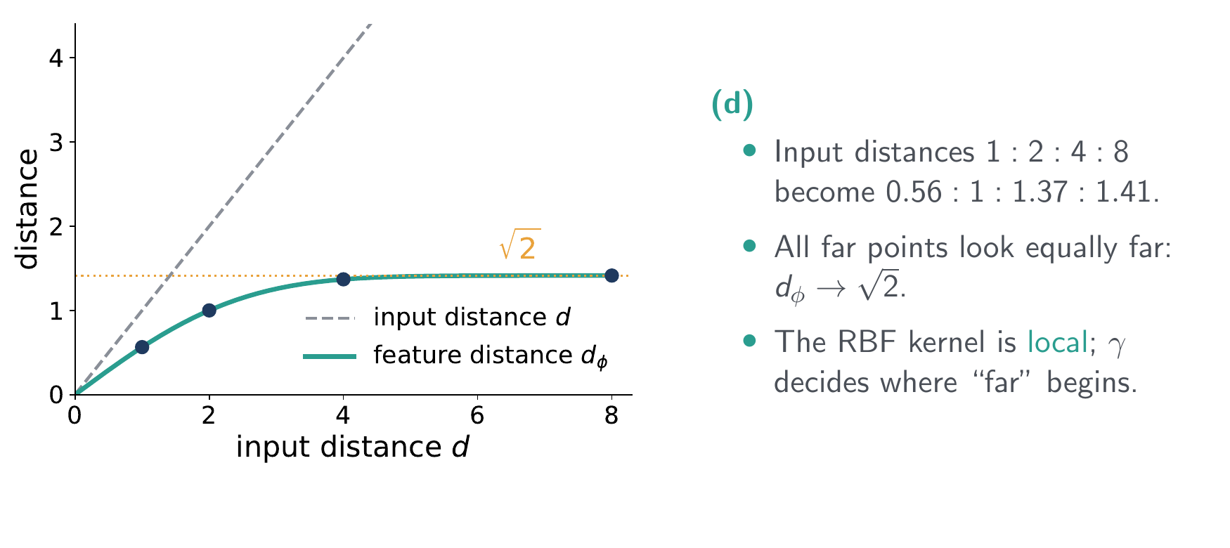
Customers compared with \(K(\mathbf x, \mathbf y) = \exp(-\gamma \|\mathbf x - \mathbf y\|^2)\). Two customers at input distance \(d = 2\) should have similarity 0.5. (a) Find \(\gamma\). (b) Show \(d_\phi^2 = 2 - 2K\). (c) Compute \(d_\phi\) for \(d = 1, 2, 4, 8\). (d) What happens to far-apart points?
- \[ e^{-4\gamma} = \tfrac12 \]
- \[ \gamma = \frac{\ln 2}{4} = 0.173 \] so \(K = 2^{-d^2/4}\).
- \(K(\mathbf x, \mathbf x) = 1\) for every point, so \[ d_\phi^2 = 1 + 1 - 2K(\mathbf x, \mathbf y) = 2 - 2K \]
-
\(d\) \(K = 2^{-d^2/4}\) \(d_\phi = \sqrt{2 - 2K}\) 1 0.841 0.564 2 0.500 1.000 4 0.0625 1.369 8 ≈ 0 1.414 - Input distances 1 : 2 : 4 : 8 become 0.56 : 1 : 1.37 : 1.41. All far points look equally far, \(d_\phi \to \sqrt 2\). The RBF kernel is local; \(\gamma\) decides where “far” begins.
Cosine similarity with the Gaussian kernel
Same \(\mathbf x = (2, 3)^T\), \(\mathbf y = (-1, 1)^T\). Find \(\cos\theta_\phi\) with the RBF kernel, \(\gamma = 0.1\).
- \[ \|\mathbf x - \mathbf y\|^2 = 3^2 + 2^2 = 13 \]
- \[ K(\mathbf x, \mathbf y) = e^{-0.1 \times 13} = e^{-1.3} = 0.2725 \]
- \[ K(\mathbf x, \mathbf x) = K(\mathbf y, \mathbf y) = 1 \]
- \[ \cos\theta_\phi = \frac{0.2725}{\sqrt{1 \times 1}} = 0.2725 \] For the RBF kernel the cosine always equals the kernel value, because every mapped point has length 1.
The mean in feature space and its length
The mean of the mapped points cannot be written down, but its length can: average all the entries of the kernel matrix. The distance from any point to that mean also comes from the kernel matrix.
- \(\mathbf 1\)
- a column of \(n\) ones; \(\mathbf 1^T \mathbf K \mathbf 1\) is the sum of all entries of \(\mathbf K\)
- \(\mathbf 1_{n \times n}\)
- the \(n \times n\) matrix of all ones (used in centring)
Expand \(\|\phi(\mathbf x_i) - \boldsymbol\mu_\phi\|^2\) like any squared distance and replace dot products by kernel values:
\[ \|\phi(\mathbf x_i) - \boldsymbol\mu_\phi\|^2 = K_{ii} - \frac2n \sum_{j=1}^n K_{ij} + \frac{1}{n^2} \sum_{k=1}^n \sum_{l=1}^n K_{kl} \]In words: the diagonal entry, minus twice the mean of row \(i\), plus the grand mean of \(\mathbf K\). This is exactly \(\hat K_{ii}\), the diagonal of the centred kernel matrix in the next card.
Norm of the feature-space mean of two points
With \(\mathbf K = \begin{bmatrix} 25 & 16 \\ 16 & 25 \end{bmatrix}\), find \(\|\boldsymbol\mu_\phi\|\) for \(\boldsymbol\mu_\phi = \tfrac12(\phi(\mathbf x_1) + \phi(\mathbf x_2))\) using only \(\mathbf K\).
- Sum of all entries: \[ \mathbf 1^T \mathbf K \mathbf 1 = 25 + 16 + 16 + 25 = 82 \]
- \[ \|\boldsymbol\mu_\phi\|^2 = \frac{82}{2^2} = 20.5 \]
- \[ \|\boldsymbol\mu_\phi\| = \sqrt{20.5} = 4.528 \]
Distance of φ(x₁) from the mean, RBF kernel
Use the RBF kernel matrix from HW2 Q5 (a): \(K_{12} = 0.3679\), \(K_{13} = 0.8642\), \(K_{23} = 0.5565\), diagonal 1.
- Mean of row 1: \[ \frac13 (1 + 0.3679 + 0.8642) = 0.7440 \]
- Grand mean: \[ \frac19 \big(3 + 2(0.3679 + 0.8642 + 0.5565)\big) = \frac{6.5772}{9} = 0.7308 \]
- \[ \|\phi(\mathbf x_1) - \boldsymbol\mu_\phi\|^2 = 1 - 2(0.7440) + 0.7308 = 0.2428 \]
- \[ \|\phi(\mathbf x_1) - \boldsymbol\mu_\phi\| = \sqrt{0.2428} = 0.4927 \]
Centring in feature space: the centred kernel matrix
PCA needs the data centred at zero. You cannot subtract the mean from vectors you never computed, but you can fix the kernel matrix instead: subtract the row means and column means and add back the grand mean.
- \(\hat{\mathbf K}\)
- centred kernel matrix: dot products of the centred feature vectors
- \(\mathbf H = \mathbf I - \frac1n \mathbf 1_{n \times n}\)
- the centring matrix; \(\hat{\mathbf K} = \mathbf H \mathbf K \mathbf H\)
- \(\bar r_i\)
- mean of row \(i\) of \(\mathbf K\) (equal to the column mean, by symmetry)
- \(\bar g\)
- mean of all \(n^2\) entries of \(\mathbf K\), which is \(\|\boldsymbol\mu_\phi\|^2\)
Recipe: centre a kernel matrix by hand
- Compute each row mean \(\bar r_i\).
- Compute the grand mean \(\bar g\) (average of the row means).
- For every entry: \[ \hat K_{ij} = K_{ij} - \bar r_i - \bar r_j + \bar g \]
- Check: every row of \(\hat{\mathbf K}\) sums to 0, and \(\hat{\mathbf K}\) is symmetric. (Rows sum to 0 because the centred vectors add up to the zero vector.)
Multiplying \(\mathbf K\) on the left by \(\frac1n \mathbf 1_{n \times n}\) replaces every entry by its column mean; on the right, by its row mean; on both sides, by the grand mean. So the four-term matrix formula and the entry-wise formula are identical. For \(n = 2\): \[ \mathbf H = \begin{bmatrix} 0.5 & -0.5 \\ -0.5 & 0.5 \end{bmatrix} \]
Quiz 2 feedback: many students skipped checking whether the data was centred. In kernel PCA the check is on \(\mathbf K\): if its rows do not sum to zero, centre it first. Eigenvalues of the uncentred \(\mathbf K\) are not variances.
Three points: K, mean norm, centred K, who is the outlier, centred cosine
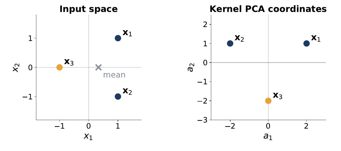
\(\mathbf x_1 = (1, 1)^T\), \(\mathbf x_2 = (1, -1)^T\), \(\mathbf x_3 = (-1, 0)^T\), kernel \((1 + \mathbf x^T \mathbf y)^2\).
- Dot products: \[ \mathbf x_1^T \mathbf x_1 = \mathbf x_2^T \mathbf x_2 = 2, \quad \mathbf x_3^T \mathbf x_3 = 1, \quad \mathbf x_1^T \mathbf x_2 = 0, \quad \mathbf x_1^T \mathbf x_3 = \mathbf x_2^T \mathbf x_3 = -1 \]
- Add 1 and square: \[ \mathbf K = \begin{bmatrix} 9 & 1 & 0 \\ 1 & 9 & 0 \\ 0 & 0 & 4 \end{bmatrix} \]
- Norm of the mean: \[ \|\boldsymbol\mu_\phi\|^2 = \frac19\, \mathbf 1^T \mathbf K \mathbf 1 = \frac{24}{9} \] so \(\|\boldsymbol\mu_\phi\| = 1.633\).
- Row means and grand mean: \[ \bar{\mathbf r} = \Big( \tfrac{10}{3},\ \tfrac{10}{3},\ \tfrac43 \Big), \quad \bar g = \tfrac83 \]
- \(\hat K_{ij} = K_{ij} - \bar r_i - \bar r_j + \bar g\), e.g. \(\hat K_{11} = 9 - \tfrac{10}3 - \tfrac{10}3 + \tfrac83 = 5\): \[ \hat{\mathbf K} = \begin{bmatrix} 5 & -3 & -2 \\ -3 & 5 & -2 \\ -2 & -2 & 4 \end{bmatrix} \]
- Squared distance to the mean in the input space, mean \((\tfrac13, 0)\): \[ \tfrac{13}{9},\ \tfrac{13}{9},\ \tfrac{16}{9} \]
- In the feature space it is \(\hat K_{ii}\): \[ 5,\ 5,\ 4 \] The ranking flips: \(\mathbf x_3\) is the outlier in the input space, \(\mathbf x_1, \mathbf x_2\) in the feature space.
- Centred cosine, centre first then normalise: \[ \cos\theta_{12} = \frac{\hat K_{12}}{\sqrt{\hat K_{11} \hat K_{22}}} = \frac{-3}{5} = -0.6 \]
Two ways to centre, and the centred kernel matrix
With \(\phi(X) = [\phi(\mathbf x_1)\ \phi(\mathbf x_2)]\) and \(\mathbf K = \begin{bmatrix} 25 & 16 \\ 16 & 25 \end{bmatrix}\): (c) can we centre with (i) \(\phi(X) - \boldsymbol\mu_\phi \mathbf 1_2^T\) or (ii) \(\phi(X)(\mathbf I - \tfrac12 \mathbf 1_{2 \times 2})\)? (d) Find \(\hat{\mathbf K}\).
- (i): \(\boldsymbol\mu_\phi \mathbf 1_2^T\) is a matrix whose two columns are both \(\boldsymbol\mu_\phi\). Subtracting it takes the mean off each column. Valid.
- (ii): \(\phi(X)\mathbf 1_{2 \times 2}\) has both columns equal to \(\phi(\mathbf x_1) + \phi(\mathbf x_2) = 2\boldsymbol\mu_\phi\). Times \(\tfrac12\), both columns are \(\boldsymbol\mu_\phi\). So (ii) is the same matrix as (i). Valid, and this is the form that leads to \(\hat{\mathbf K} = \mathbf H \mathbf K \mathbf H\).
- Row means: both \(\tfrac{41}{2} = 20.5\). Grand mean 20.5.
- \[ \hat K_{11} = 25 - 20.5 - 20.5 + 20.5 = 4.5 \]
- \[ \hat K_{12} = 16 - 20.5 - 20.5 + 20.5 = -4.5 \]
- \[ \hat{\mathbf K} = \begin{bmatrix} 4.5 & -4.5 \\ -4.5 & 4.5 \end{bmatrix} \] Rows sum to 0 ✓
Centre K = [[1, 1], [1, 4]]
- Row means: \(\bar r_1 = 1\), \(\bar r_2 = 2.5\). Grand mean \(\bar g = \tfrac14(1 + 1 + 1 + 4) = 1.75\).
- \[ \hat K_{11} = 1 - 1 - 1 + 1.75 = 0.75 \]
- \[ \hat K_{12} = 1 - 1 - 2.5 + 1.75 = -0.75 \]
- \[ \hat K_{22} = 4 - 2.5 - 2.5 + 1.75 = 0.75 \]
- \[ \hat{\mathbf K} = \begin{bmatrix} 0.75 & -0.75 \\ -0.75 & 0.75 \end{bmatrix} \] The grading scheme gave 1 point for the means, 1.5 for the three distinct entries, 0.5 for the final matrix.
Part 4
Kernel PCA
PCA recap, written with points as columns
This is the PCA you already know, but with the data stored as columns and the covariance written as a matrix product. Kernel PCA rewrites each of these lines using the kernel matrix.
Rows-as-samples there, columns-as-samples here. With columns, \(\frac1n X X^T\) is the covariance; with rows it is \(\frac1n X^T X\). Everything else is identical: see PCA as an optimisation and the PCA algorithm on the Lectures 3–4 page.
Kernel PCA: the idea and the obstacle
Do ordinary PCA, but on the mapped and centred points. The problem is that the covariance matrix in feature space is huge or infinite, so every step must be rewritten using the small n×n centred kernel matrix.
- \(\boldsymbol\Sigma_\phi\)
- covariance of the centred feature vectors (size: feature dimension squared)
- \(\lambda\)
- variance along a principal direction in feature space
- \(\mathbf u\)
- a principal direction in feature space (we will never write it explicitly)
Derivation: from Σφu = λu to K̂c = ηc
Each principal direction is a weighted sum of the data points, so finding it means finding n weights. Dotting the eigen-equation with each data point turns everything into kernel values, and the weights come out as an eigenvector of the centred kernel matrix.
Step I: every direction is a weighted sum of the points
Step II: substitute and meet K̂
Step III: dot with each point to get numbers
Cancel one \(\hat{\mathbf K}\) from both sides of \(\frac1n \hat{\mathbf K}^2 \mathbf c = \lambda \hat{\mathbf K} \mathbf c\) and multiply by \(n\). The result is a plain eigenproblem for the \(n \times n\) matrix \(\hat{\mathbf K}\). Its eigenvalue \(\eta\) is \(n\) times the variance \(\lambda\).
Step IV: unit length and the coordinates
- \(\mathbf v\)
- unit eigenvector of \(\hat{\mathbf K}\) (length 1, what you get from the characteristic equation)
- \(\mathbf c\)
- the same eigenvector rescaled to length \(1/\sqrt\eta\), so that \(\mathbf u\) has length 1
- \(\mathbf a\)
- the \(n\) coordinates of the training points on this component
For the training points you never need \(\mathbf c\): the coordinates are the unit eigenvector times the square root of its eigenvalue.
\[ \mathbf a_i = \sqrt{\eta_i}\, \mathbf v_i \]Check: the variance of the coordinates is \(\frac1n \|\mathbf a\|^2 = \frac1n \eta \|\mathbf v\|^2 = \eta / n = \lambda\), as it should be. Quiz 2 P2(d) was exactly this line.
PCA vs kernel PCA, and the linear kernel
Side by side, every PCA quantity has a kernel twin. With the linear kernel the twins are literally the same numbers, which is also a cheap way to do PCA when there are far more attributes than points.
Centring makes the \(n\) feature vectors add up to zero, so they span at most \(n - 1\) directions. One eigenvalue of \(\hat{\mathbf K}\) is always 0, with eigenvector \((1, 1, \dots, 1)^T\). With \(n = 2\) points there is exactly one component (HW2 Q3, Quiz 2); with \(n = 3\), two (L6 Example 3).
The kernel PCA algorithm
Build the kernel matrix, centre it, find its eigenvalues and unit eigenvectors, and scale each eigenvector by the square root of its eigenvalue to get the new coordinates.
Recipe for an exam question (n = 2 or 3 points)
- Dot products of the points, then apply the kernel formula to each: \(\mathbf K\).
- Row means and grand mean, then \(\hat K_{ij} = K_{ij} - \bar r_i - \bar r_j + \bar g\). Check rows sum to 0.
- Eigenvalues of \(\hat{\mathbf K}\) from \(\det(\hat{\mathbf K} - \eta \mathbf I) = 0\). One of them is 0. Unit eigenvectors \(\mathbf v_i\).
- Variances in feature space: \(\lambda_i = \eta_i / n\). Fraction kept by the first component: \(\eta_1 / \sum \eta_i\).
- Coordinates of the training points on component \(i\): \(\mathbf a_i = \sqrt{\eta_i}\, \mathbf v_i\). Check: \(\frac1n \|\mathbf a_i\|^2 = \lambda_i\), and \(a_{1}^2 + a_{2}^2 + \dots = \hat K_{jj}\) for each point \(j\) when all components are kept.
Reporting \(\eta\) as the variance (it is \(\eta / n\)). Using the unit eigenvector as the coordinates (multiply by \(\sqrt\eta\)). Working with the uncentred \(\mathbf K\) (HW2 Q5c asks for the dominant eigenvector of \(\mathbf K\) itself; that is a matrix exercise, not kernel PCA).
Kernel PCA on Example 3, by hand
Start from the centred matrix of Example 3:
\[ \hat{\mathbf K} = \begin{bmatrix} 5 & -3 & -2 \\ -3 & 5 & -2 \\ -2 & -2 & 4 \end{bmatrix} \]- Eigenvectors from symmetry. Swapping \(\mathbf x_1 \leftrightarrow \mathbf x_2\) leaves \(\hat{\mathbf K}\) unchanged, so try \((1, -1, 0)^T\): \[ \hat{\mathbf K} \begin{bmatrix} 1 \\ -1 \\ 0 \end{bmatrix} = \begin{bmatrix} 8 \\ -8 \\ 0 \end{bmatrix} \] so \(\eta_1 = 8\).
- \[ \hat{\mathbf K} \begin{bmatrix} 1 \\ 1 \\ -2 \end{bmatrix} = \begin{bmatrix} 6 \\ 6 \\ -12 \end{bmatrix} \] so \(\eta_2 = 6\).
- \[ \hat{\mathbf K} \begin{bmatrix} 1 \\ 1 \\ 1 \end{bmatrix} = \begin{bmatrix} 0 \\ 0 \\ 0 \end{bmatrix} \] so \(\eta_3 = 0\).
- Variances: \[ \lambda_1 = \tfrac83, \quad \lambda_2 = 2 \]
- Fraction of variance: \[ \tfrac{8}{14} = 57\%, \quad \tfrac{6}{14} = 43\% \] Two components capture 100%. With \(n = 3\) points at most \(n - 1 = 2\) can be nonzero.
- Scaling \(\mathbf c_i = \mathbf v_i / \sqrt{\eta_i}\): \[ \mathbf c_1 = \frac{1}{\sqrt 2} \frac{1}{\sqrt 8} \begin{bmatrix} 1 \\ -1 \\ 0 \end{bmatrix} = \frac14 \begin{bmatrix} 1 \\ -1 \\ 0 \end{bmatrix} \]
- \[ \mathbf c_2 = \frac{1}{\sqrt 6} \frac{1}{\sqrt 6} \begin{bmatrix} 1 \\ 1 \\ -2 \end{bmatrix} = \frac16 \begin{bmatrix} 1 \\ 1 \\ -2 \end{bmatrix} \]
- Coordinates \(\mathbf a_i = \hat{\mathbf K} \mathbf c_i\): \[ \mathbf a_1 = \frac14 \begin{bmatrix} 8 \\ -8 \\ 0 \end{bmatrix} = \begin{bmatrix} 2 \\ -2 \\ 0 \end{bmatrix} \]
- \[ \mathbf a_2 = \frac16 \begin{bmatrix} 6 \\ 6 \\ -12 \end{bmatrix} = \begin{bmatrix} 1 \\ 1 \\ -2 \end{bmatrix} \]
- Check the variances: \[ \tfrac13 (2^2 + 2^2 + 0^2) = \tfrac83 = \lambda_1 \]
- \[ \tfrac13 (1^2 + 1^2 + 2^2) = 2 = \lambda_2 \]
- PC 1 separates \(\mathbf x_1\) from \(\mathbf x_2\); PC 2 separates \(\mathbf x_3\) from the pair. In the input space \(\mathbf x_3\) looked like the outlier; kernel PCA spreads all three points apart.
Eigenvalues, variances and coordinates for two points
From \(\hat{\mathbf K} = \begin{bmatrix} 4.5 & -4.5 \\ -4.5 & 4.5 \end{bmatrix}\): (e) all eigenvalues and eigenvectors of \(\hat{\mathbf K}\); (f) eigenvalues of \(\boldsymbol\Sigma_\phi\); (g) coordinates of the centred \(\phi(\mathbf x_1)\), \(\phi(\mathbf x_2)\) along the eigenvectors of \(\boldsymbol\Sigma_\phi\).
- \[ \det(\hat{\mathbf K} - \eta \mathbf I) = (4.5 - \eta)^2 - 4.5^2 = 0 \]
- \[ \eta (\eta - 9) = 0 \]
- \[ \eta_1 = 9, \quad \eta_2 = 0 \]
- For \(\eta_1 = 9\): \((4.5 - 9) v_1 - 4.5 v_2 = 0\) gives \(v_2 = -v_1\). \[ \mathbf v_1 = \frac{1}{\sqrt 2} \begin{bmatrix} 1 \\ -1 \end{bmatrix} \]
- For \(\eta_2 = 0\): \(v_2 = v_1\). \[ \mathbf v_2 = \frac{1}{\sqrt 2} \begin{bmatrix} 1 \\ 1 \end{bmatrix} \]
- Eigenvalues of \(\boldsymbol\Sigma_\phi\): \[ \lambda_1 = \frac{9}{2} = 4.5, \quad \lambda_2 = 0 \] (all remaining feature-space directions also have eigenvalue 0).
- Coordinates on the first component: \[ \mathbf a_1 = \sqrt{\eta_1}\, \mathbf v_1 = \frac{3}{\sqrt 2} \begin{bmatrix} 1 \\ -1 \end{bmatrix} = \begin{bmatrix} 2.121 \\ -2.121 \end{bmatrix} \] On the second, both coordinates are 0.
- Check: \(a_{11}^2 = 4.5 = \hat K_{11}\) ✓ and \(\tfrac12(2.121^2 + 2.121^2) = 4.5 = \lambda_1\) ✓. The key reports the same values with the opposite sign, which is also correct.
Eigen-decompose the centred K and project
From \(\hat{\mathbf K} = \begin{bmatrix} 0.75 & -0.75 \\ -0.75 & 0.75 \end{bmatrix}\): (c) eigenvalues and unit eigenvectors of \(\hat{\mathbf K}\), and the eigenvalues of \(\boldsymbol\Sigma_\phi\); (d) the coordinate of each point on the first kernel principal component.
- \[ \det(\hat{\mathbf K} - \eta \mathbf I) = (0.75 - \eta)^2 - 0.75^2 = \eta(\eta - 1.5) = 0 \]
- \[ \eta_1 = 1.5, \quad \mathbf c_1 = \tfrac{1}{\sqrt 2}(1, -1)^T \]
- \[ \eta_2 = 0, \quad \mathbf c_2 = \tfrac{1}{\sqrt 2}(1, 1)^T \]
- Eigenvalues of \(\boldsymbol\Sigma_\phi\): \[ \frac{1.5}{2} = 0.75, \quad 0 \]
- \[ a_{11} = \sqrt{1.5} \times \tfrac{1}{\sqrt 2} = \sqrt{0.75} = 0.866, \quad a_{21} = -0.866 \]
- Check: \(\hat K_{11} = \|\hat\phi(\mathbf x_1)\|^2 = 0.75 = a_{11}^2\), consistent with all variance lying along one direction. Opposite signs accepted. (Grading: 1.5 for the eigenvalues of \(\hat{\mathbf K}\), 1.5 for unit eigenvectors, 1 for the eigenvalues of \(\boldsymbol\Sigma_\phi\), 1 per coordinate.)
Dominant eigenvector of the (uncentred) RBF kernel matrix
For \(\mathbf K = \begin{bmatrix} 1 & 0.3679 & 0.8642 \\ 0.3679 & 1 & 0.5565 \\ 0.8642 & 0.5565 & 1 \end{bmatrix}\), find the dominant eigenvalue and eigenvector.
- A 3×3 characteristic polynomial is not an exam-size task; the 2025 key used software. \[ \eta_{\max} = 2.2176, \quad \mathbf v_{\max} = (0.6002,\ 0.4754,\ 0.6433)^T \]
- How to verify any claimed pair: multiply. \[ \mathbf K \mathbf v_{\max} = (1.331,\ 1.054,\ 1.427)^T \] and \(2.2176 \times \mathbf v_{\max} = (1.331,\ 1.054,\ 1.427)^T\). They agree.
- All three entries of \(\mathbf v_{\max}\) are positive and similar in size: the dominant eigenvector of an uncentred similarity matrix mostly measures “how similar each point is to everyone”, not a principal direction. For kernel PCA you would centre \(\mathbf K\) first.
Part 5
Exam toolkit
Which formula, when
The formulas are given in the exam. The skill tested is picking the right one and showing the steps.
| The question asks for… | Use | Card |
|---|---|---|
| the feature vector \(\phi(\mathbf x)\) of a quadratic kernel | squares, then \(\sqrt 2\) × each product (and \(\sqrt{2c}\, x_i\), \(c\) if \(c \ne 0\)) | Feature map Kernel functions |
| a kernel value | \((c + \mathbf x^T \mathbf y)^p\) or \(\exp(-\gamma \|\mathbf x - \mathbf y\|^2)\) | Kernel functions |
| the kernel matrix | Gram matrix \(X^T X\), then the kernel formula entry by entry | Kernel matrix |
| is this matrix a valid kernel? | symmetric, diagonal ≥ 0, no negative eigenvalue | Kernel matrix |
| length of \(\phi(\mathbf x)\) | \(\sqrt{K(\mathbf x, \mathbf x)}\) | Norm, distance, cosine |
| distance between \(\phi(\mathbf x)\) and \(\phi(\mathbf y)\) | \(\sqrt{K(\mathbf x,\mathbf x) + K(\mathbf y,\mathbf y) - 2K(\mathbf x,\mathbf y)}\) | Norm, distance, cosine |
| cosine similarity in feature space | \(K(\mathbf x,\mathbf y) / \sqrt{K(\mathbf x,\mathbf x) K(\mathbf y,\mathbf y)}\) | Norm, distance, cosine |
| norm of the feature-space mean | \(\sqrt{\tfrac{1}{n^2} \mathbf 1^T \mathbf K \mathbf 1}\) (root of the grand mean) | Mean in feature space |
| distance of a point from the mean | \(\sqrt{K_{ii} - 2 \bar r_i + \bar g} = \sqrt{\hat K_{ii}}\) | Mean in feature space |
| the centred kernel matrix | \(\hat K_{ij} = K_{ij} - \bar r_i - \bar r_j + \bar g\), or \(\mathbf H \mathbf K \mathbf H\) | Centring K |
| variance along a kernel component | \(\lambda = \eta / n\), with \(\eta\) an eigenvalue of \(\hat{\mathbf K}\) | Dot with each point |
| coordinates of the points on a component | \(\mathbf a = \sqrt\eta\, \mathbf v\) (or \(\hat{\mathbf K} \mathbf c\) with \(\mathbf c = \mathbf v / \sqrt\eta\)) | Scaling & coordinates |
| how many components to keep | smallest \(r\) with \(\sum_{i \le r} \eta_i / \sum \eta_i \ge \alpha\); at most \(n - 1\) | Kernel PCA algorithm |
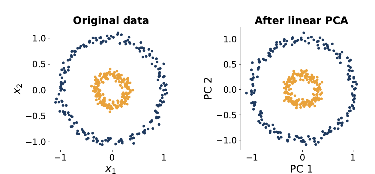
| why ordinary PCA failed on this data | PCA only rotates; a curve or a ring needs a nonlinear feature | Linear PCA misses curves |
Rows of \(\hat{\mathbf K}\) sum to 0. One eigenvalue of \(\hat{\mathbf K}\) is 0. The kernel variances \(\eta_i / n\) add up to the mean of the diagonal of \(\hat{\mathbf K}\). For an RBF kernel every diagonal entry of \(\mathbf K\) is 1 and every entry lies in \((0, 1]\).