Linear regression
Lecture 7 (Linear Regression I), rebuilt as one storyline: the model, the line, the geometry behind it, and the matrix formula that covers every case.
How to read this page. It is ordered by concept, not by slide. Each card says which slides it came from, what to read first, and what uses it later.
Teal = explanation added by Claude, not on the slides. Amber = watch out. Dropdowns hide worked examples, practice questions, and their answers.
The road to the regression formula
RMSE, residual plots and the Iris examples are side stops: useful for interpreting a fit, but the main chain does not need them.
Lecture map: which slides each card covers
Part 1
From unsupervised to supervised
The regression model: a target plus noise
Until now we only had a data table and looked for structure in it. Now each row also has an answer, and we want a rule that predicts the answer for new rows.
- \(X_1,\dots,X_d\)
- predictors (inputs), \(d\) of them
- \(Y\)
- response (the thing to predict)
- \(f(\mathbf X)\)
- the part of \(Y\) explained by the predictors
- \(\varepsilon\)
- random error, independent of \(\mathbf X\): measurement noise plus everything not measured (latent variables)
- \(n\)
- number of training rows
Delivery time depends on distance, but also on traffic, weather and the driver. What we do not measure ends up in \(\varepsilon\). The slides' examples: food delivery (distance, stops → time), power grid (temperature, hour → load), real estate (area, rooms → price), language models (compute → test loss).
Part 2
The line and the error
The linear model: bias plus weights
We guess that the answer is a weighted sum of the inputs plus a constant. With one input it is a straight line, with two it is a flat plane.
- \(b\)
- bias or intercept: the prediction when every input is 0
- \(w_i\)
- regression coefficient (weight) of \(X_i\): how much \(\hat y\) changes per unit of \(X_i\)
- \(\hat y_i\)
- predicted value for row \(i\) (hat = fitted, not observed)
- \(\epsilon_i\)
- residual: observed minus predicted, for row \(i\)
\(\varepsilon\) in the model is the true, unknown noise. \(\epsilon_i = y_i - \hat y_i\) is the residual you can compute after fitting. The residual is our estimate of the noise.
Least squares: pick the line with the smallest squared error
There are many possible lines. We choose the one whose total squared miss, added over all points, is smallest.
Because SSE is a smooth bowl in \(b\) and \(\mathbf w\), setting its derivatives to zero gives the minimum directly. Every formula on this page comes from doing exactly that.
Part 3
One predictor
One predictor: intercept and slope
For one input, the best line always goes through the point of averages, and its slope is the covariance of the two variables divided by the variance of the input.
Intercept: set the derivative with respect to \(b\) to zero
Slope: set the derivative with respect to \(w\) to zero
- \(\mu_X, \mu_Y\)
- sample means of the input and the response
- \(\sigma_{XY}\)
- sample covariance of \(X\) and \(Y\)
- \(\sigma_X^2\)
- sample variance of \(X\)
Recipe: fit a line by hand
- Compute \(\mu_X\) and \(\mu_Y\).
- Make a table with columns \(x_i - \mu_X\), \(y_i - \mu_Y\), \((x_i - \mu_X)^2\), \((x_i-\mu_X)(y_i-\mu_Y)\).
- \[ w = \frac{\sum (x_i - \mu_X)(y_i - \mu_Y)}{\sum (x_i - \mu_X)^2} \]
- \[ b = \mu_Y - w\,\mu_X \]
- Write the line \(\hat y = b + w x\) and use it to predict.
The slope is a ratio of a covariance to a variance. Whether both use \(1/n\) or \(1/(n-1)\), the factor cancels. The sums in the table need no division at all.
Delivery times: fit the line by hand and predict 7 km
A delivery company records five orders in Doha. How long should a 7 km order take?
| Order | \(x\) (km) | \(y\) (min) |
|---|---|---|
| 1 | 2 | 15 |
| 2 | 4 | 16 |
| 3 | 6 | 24 |
| 4 | 8 | 30 |
| 5 | 10 | 35 |
- \[ \mu_X = \frac{30}{5} = 6 \]
- \[ \mu_Y = \frac{120}{5} = 24 \]
- Deviation table:
\(x_i\) \(y_i\) \(x_i - \mu_X\) \(y_i - \mu_Y\) \((x_i-\mu_X)^2\) \((x_i-\mu_X)(y_i-\mu_Y)\) 2 15 −4 −9 16 36 4 16 −2 −8 4 16 6 24 0 0 0 0 8 30 2 6 4 12 10 35 4 11 16 44 sum 40 108 - \[ w = \frac{108}{40} = 2.7 \]
- \[ b = 24 - 2.7 \times 6 = 7.8 \]
- \[ \hat y = 7.8 + 2.7\,x \]
- \[ \hat y(7) = 7.8 + 2.7 \times 7 = 26.7 \text{ min} \]
Interpretation (s11): each extra km adds about 2.7 minutes; 7.8 min is the fixed time per order (pickup, parking). Predicting at 30 km is extrapolation: there is no data there.
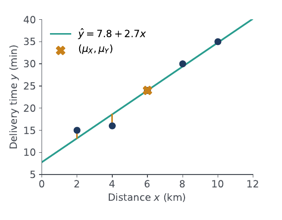
Same delivery line from the covariance numbers alone
Using \(1/n\), the delivery data has \(\sigma_X^2 = 8\) and \(\sigma_{XY} = 21.6\), with \(\mu_X = 6\) and \(\mu_Y = 24\). Find the line without the table, then check against the slide.
- \[ w = \frac{\sigma_{XY}}{\sigma_X^2} = \frac{21.6}{8} = 2.7 \]
- \[ b = 24 - 2.7 \times 6 = 7.8 \]
- Same line as the slide. The sums 108 and 40 divided by \(n = 5\) are 21.6 and 8, so the ratio is unchanged.
Residuals and their two zero-sum identities
A residual is how far each point sits above or below the line. For a least-squares line, the residuals always add up to zero and are not correlated with the input.
Setting \(\partial\,\mathrm{SSE}/\partial b = 0\) is the same as \(\sum \epsilon_i = 0\). Setting \(\partial\,\mathrm{SSE}/\partial w = 0\) is the same as \(\sum x_i \epsilon_i = 0\). The geometry card residuals are orthogonal says the same thing with vectors.
Delivery residuals and SSE
| \(x_i\) | \(y_i\) | \(\hat y_i\) | \(\epsilon_i = y_i - \hat y_i\) |
|---|---|---|---|
| 2 | 15 | 13.2 | 1.8 |
| 4 | 16 | 18.6 | −2.6 |
| 6 | 24 | 24.0 | 0.0 |
| 8 | 30 | 29.4 | 0.6 |
| 10 | 35 | 34.8 | 0.2 |
- \[ \mathrm{SSE} = 3.24 + 6.76 + 0 + 0.36 + 0.04 \]
- \[ \mathrm{SSE} = 10.4 \]
- Check one: \[ \sum_i \epsilon_i = 1.8 - 2.6 + 0 + 0.6 + 0.2 = 0 \]
- Check two: \[ \sum_i x_i \epsilon_i = 3.6 - 10.4 + 0 + 4.8 + 2.0 = 0 \]
Root mean squared error: a typical miss in the units of \(Y\)
SSE grows with the number of points and is in squared units. RMSE fixes both, so it tells you how far off a typical prediction is.
Delivery RMSE
- \[ \mathrm{RMSE} = \sqrt{\frac{10.4}{5}} \]
- \[ \mathrm{RMSE} = \sqrt{2.08} = 1.44 \text{ min} \]
A typical prediction is off by about 1.4 minutes.
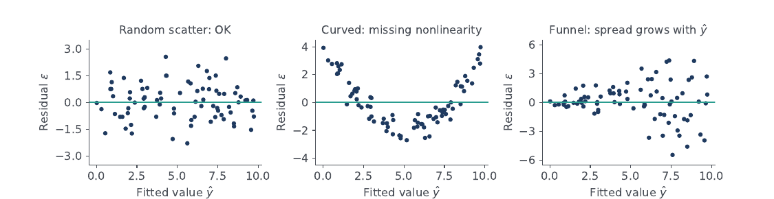
Residual plots: what a good fit looks like
Plot each residual against its prediction. If you can see a shape, the straight line is missing something, no matter how small the error number is.
Iris: petal width from petal length
The same recipe on 150 flowers. The numbers are bigger, but the only inputs are the two means, one variance and one covariance.
The slides use the original UCI Iris file. scikit-learn's copy corrects two entries, so its means, slope and SSE differ in the third decimal (s32 says so). In an exam, use the numbers the question gives you.
Part 4
The geometry: least squares is a projection
This part explains why the formulas work. It is also the route HW2 Q6 asks for.
Two views of the data: rows as points, columns as vectors
So far each order was a dot on a 2-D plot. Now flip it: each variable becomes one long vector with one entry per order, and fitting a line means choosing one vector.
- \(\mathbf 1\)
- the vector of \(n\) ones (it carries the intercept)
- \(X, Y\)
- capital letters now mean the whole column of \(n\) values
- \(\operatorname{span}\{\mathbf 1, X\}\)
- every vector of the form \(b\mathbf 1 + wX\): a 2-D plane inside \(\mathbb R^n\)
Least squares = orthogonal projection of \(Y\) onto the plane
The data vector is not in the plane because the data are noisy. The closest point in the plane is found by dropping a perpendicular, and that closest point is the fitted vector.
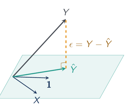
Projecting onto a unit vector was card “Projection” on the Lectures 3–4 page. The only new thing is that the target is a plane with two directions, and they are not at right angles, so we first split them.
Make the two directions orthogonal, then project onto each
\(Y^T \bar X = \sum (y_i)(x_i - \mu_X)\) equals \(\sum (y_i - \mu_Y)(x_i - \mu_X)\) because \(\bar X\) sums to zero. And \(\bar X^T \bar X = \sum (x_i - \mu_X)^2\). So \(w\) is the covariance-over-variance slope again.
What the perpendicular residual means
Recipe: the “geometric approach” a question may ask for
- Write \(\mathbf 1\), \(X\) and \(Y\) as column vectors of length \(n\).
- Form \(A = [\mathbf 1 \; X]\) and compute \(A^T A\) and \(A^T Y\).
- Solve \((A^T A)\,(b, w)^T = A^T Y\) with the 2×2 inverse (next part has the formula).
- \[ \hat Y = A\,(b, w)^T = b\,\mathbf 1 + w\,X \]
- Check: \(\boldsymbol\epsilon = Y - \hat Y\) sums to zero and \(X^T \boldsymbol\epsilon = 0\).
Predicted vector and the line by the geometric approach
Data: \(X = (5, 0, 2, 1, 2)\), \(Y = (2, 1, 1, 1, 0)\). (a) Compute the predicted response vector \(\hat Y\) for least-squares regression using the geometric approach. (b) Extract the bias and slope and give the equation of the best-fitting line.
- \[ A = [\mathbf 1 \; X] = \begin{bmatrix}1&5\\1&0\\1&2\\1&1\\1&2\end{bmatrix} \]
- Sums: \(\sum x_i = 10\), \(\sum x_i^2 = 34\), \(\sum y_i = 5\), \(\sum x_i y_i = 13\).
- \[ A^T A = \begin{bmatrix} n & \sum x_i \\ \sum x_i & \sum x_i^2 \end{bmatrix} = \begin{bmatrix}5&10\\10&34\end{bmatrix} \]
- \[ A^T Y = \begin{bmatrix} \sum y_i \\ \sum x_i y_i \end{bmatrix} = \begin{bmatrix}5\\13\end{bmatrix} \]
- \[ \det(A^T A) = 5 \times 34 - 10 \times 10 = 70 \]
- \[ (A^T A)^{-1} = \frac{1}{70} \begin{bmatrix}34&-10\\-10&5\end{bmatrix} \]
- \[ \begin{bmatrix} b \\ w \end{bmatrix} = \frac{1}{70} \begin{bmatrix}34&-10\\-10&5\end{bmatrix} \begin{bmatrix}5\\13\end{bmatrix} = \frac{1}{70} \begin{bmatrix}170 - 130\\-50 + 65\end{bmatrix} \]
- \[ \begin{bmatrix} b \\ w \end{bmatrix} = \begin{bmatrix} 4/7 \\ 3/14 \end{bmatrix} = \begin{bmatrix} 0.5714 \\ 0.2143 \end{bmatrix} \]
- \[ \hat Y = \frac47 \mathbf 1 + \frac{3}{14} X = \begin{bmatrix} 23/14 \\ 4/7 \\ 1 \\ 11/14 \\ 1 \end{bmatrix} = \begin{bmatrix} 1.6429 \\ 0.5714 \\ 1.0000 \\ 0.7857 \\ 1.0000 \end{bmatrix} \]
- (b) Bias \(b = 4/7 = 0.5714\), slope \(w = 3/14 = 0.2143\): \[ \hat y = 0.5714 + 0.2143\,x \]
- Check: residuals \(Y - \hat Y = (0.3571, 0.4286, 0, 0.2143, -1)\) sum to 0, and \(X^T \boldsymbol\epsilon = 1.7857 + 0 + 0 + 0.2143 - 2 = 0\).
\(\mu_X = 2\), \(\mu_Y = 1\), \(\sum (x_i-2)(y_i-1) = 3\), \(\sum (x_i - 2)^2 = 14\), so \(w = 3/14\) and \(b = 1 - (3/14)(2) = 4/7\). Both routes agree; the question says “geometric”, so show the matrix route for credit.
Part 5
Multiple regression
Absorb the bias: one weight vector for all \(d + 1\) parameters
Add a column of ones to the data, and the intercept becomes just another weight. Then one matrix formula covers one predictor, two, or a hundred.
- \(\tilde D\)
- the data matrix with a column of ones in front (tilde = augmented)
- \(\tilde{\mathbf w}\)
- bias first, then the \(d\) weights
- \(\tilde{\mathbf x}_i\)
- row \(i\) of \(\tilde D\), i.e. \((1, x_{i1}, \dots, x_{id})^T\)
With \(d = 1\), \(\tilde D\) is exactly the matrix \(A = [\mathbf 1 \; X]\) from the projection card. HW2 Q6 calls it \(A\).
Normal equations: the closed-form solution
Write SSE with matrices, set its gradient to zero, and the best weights come out of one matrix inverse. This is the formula the exam will give you.
- \(\tilde D^T \tilde D\)
- \((d+1) \times (d+1)\) matrix of sums of products of the columns
- \(\tilde D^T Y\)
- vector of sums of products of each column with \(Y\)
Recipe: normal equations by hand
- Build \(\tilde D\) by putting a column of ones before the predictors.
- Compute \(\tilde D^T \tilde D\): entry \((j,k)\) is the dot product of columns \(j\) and \(k\). The top-left entry is \(n\).
- Compute \(\tilde D^T Y\): entry \(j\) is the dot product of column \(j\) with \(Y\).
- Invert \(\tilde D^T \tilde D\) (2×2 by formula; 3×3 only if the question makes it easy) and multiply.
- Read off \(b\) first, then \(w_1, \dots, w_d\).
If one predictor is a copy or an exact combination of others (for example temperature in °C and in °F), \(\tilde D^T \tilde D\) is singular and there is no unique \(\tilde{\mathbf w}\). Nearly-dependent predictors are the topic of the correlated predictors card.
Hand calculation with centred data
Subtract the means first and the intercept drops out of the matrix. With two predictors you only need to invert a 2×2 matrix, then get the bias from the means.
- \(\bar D\)
- \(n \times d\) matrix of centred predictors (no column of ones)
- \(\boldsymbol\mu_X\)
- vector of the \(d\) predictor means
- \(\Sigma\)
- covariance matrix of the predictors, with \(1/n\)
Recipe: two predictors by hand
- Compute the means \(\mu_1, \mu_2, \mu_Y\) and centre all three columns.
- \[ \bar D^T \bar D = \begin{bmatrix} \sum \bar x_{i1}^2 & \sum \bar x_{i1}\bar x_{i2} \\ \sum \bar x_{i1}\bar x_{i2} & \sum \bar x_{i2}^2 \end{bmatrix} \]
- \[ \bar D^T \bar Y = \begin{bmatrix} \sum \bar x_{i1} \bar y_i \\ \sum \bar x_{i2} \bar y_i \end{bmatrix} \]
- Invert the 2×2 with the formula and multiply to get \(\mathbf w = (w_1, w_2)^T\).
- \[ b = \mu_Y - w_1 \mu_1 - w_2 \mu_2 \]
With one predictor, \(w = \sigma_{XY}/\sigma_X^2\). With two, do not divide covariances one at a time; the inverse matrix mixes them. Dividing separately is only correct when the two predictors are uncorrelated (off-diagonal entry 0).
Delivery time from distance and number of stops
The company also records how many stops each driver made. Fit \(\hat y = b + w_1 x_1 + w_2 x_2\).
| Distance \(x_1\) | Stops \(x_2\) | Time \(y\) | \(x_1 - 6\) | \(x_2 - 2\) | \(y - 24\) |
|---|---|---|---|---|---|
| 2 | 1 | 15 | −4 | −1 | −9 |
| 4 | 1 | 16 | −2 | −1 | −8 |
| 6 | 2 | 24 | 0 | 0 | 0 |
| 8 | 3 | 30 | 2 | 1 | 6 |
| 10 | 3 | 35 | 4 | 1 | 11 |
- Means: \(\mu_1 = 6\), \(\mu_2 = 2\), \(\mu_Y = 24\) (the centred columns are in the table).
- \[ \bar D^T \bar D = \begin{bmatrix} 40 & 12 \\ 12 & 4 \end{bmatrix} \]
- \[ \bar D^T \bar Y = \begin{bmatrix} 108 \\ 34 \end{bmatrix} \]
- \[ \det = 40 \times 4 - 12 \times 12 = 160 - 144 = 16 \]
- \[ (\bar D^T \bar D)^{-1} = \frac{1}{16} \begin{bmatrix} 4 & -12 \\ -12 & 40 \end{bmatrix} \]
- \[ \mathbf w = \frac{1}{16} \begin{bmatrix} 4 \cdot 108 - 12 \cdot 34 \\ -12 \cdot 108 + 40 \cdot 34 \end{bmatrix} = \frac{1}{16} \begin{bmatrix} 24 \\ 64 \end{bmatrix} \]
- \[ \mathbf w = \begin{bmatrix} 1.5 \\ 4 \end{bmatrix} \]
- \[ b = 24 - 1.5 \times 6 - 4 \times 2 = 7 \]
- \[ \hat y = 7 + 1.5\,x_1 + 4\,x_2 \]
Interpreting the coefficients (s28):
| Model | Weight of distance | SSE | RMSE (min) |
|---|---|---|---|
| Distance only | 2.7 | 10.4 | 1.44 |
| Distance + stops | 1.5 | 4.0 | 0.89 |
- \(w_1 = 1.5\): one extra km adds 1.5 min when the number of stops is held fixed.
- \(w_2 = 4\): each extra stop adds 4 min at the same distance.
- Longer trips had more stops, so the simple model gave distance credit for the stops.
A coefficient's meaning depends on which other predictors are in the model.
Two predictors, four rows, by hand
\(x_1 = (1, 2, 3, 4)\), \(x_2 = (2, 1, 4, 3)\), \(y = (5, 6, 10, 12)\). Fit \(\hat y = b + w_1 x_1 + w_2 x_2\) with the centred method, then find the SSE.
- Means: \(\mu_1 = 2.5\), \(\mu_2 = 2.5\), \(\mu_Y = 8.25\).
- Centred columns: \(\bar x_1 = (-1.5, -0.5, 0.5, 1.5)\), \(\bar x_2 = (-0.5, -1.5, 1.5, 0.5)\), \(\bar y = (-3.25, -2.25, 1.75, 3.75)\).
- \[ \bar D^T \bar D = \begin{bmatrix} 5 & 3 \\ 3 & 5 \end{bmatrix} \]
- \[ \bar D^T \bar Y = \begin{bmatrix} 12.5 \\ 9.5 \end{bmatrix} \]
- \[ \det = 25 - 9 = 16 \]
- \[ (\bar D^T \bar D)^{-1} = \frac{1}{16} \begin{bmatrix} 5 & -3 \\ -3 & 5 \end{bmatrix} \]
- \[ \mathbf w = \frac{1}{16} \begin{bmatrix} 62.5 - 28.5 \\ -37.5 + 47.5 \end{bmatrix} = \frac{1}{16} \begin{bmatrix} 34 \\ 10 \end{bmatrix} = \begin{bmatrix} 2.125 \\ 0.625 \end{bmatrix} \]
- \[ b = 8.25 - 2.125 \times 2.5 - 0.625 \times 2.5 = 1.375 \]
- \[ \hat y = 1.375 + 2.125\,x_1 + 0.625\,x_2 \]
- Predictions \((4.75, 6.25, 10.25, 11.75)\), residuals \((0.25, -0.25, -0.25, 0.25)\).
- \[ \mathrm{SSE} = 4 \times 0.0625 = 0.25 \]
Iris with two predictors: a fitted plane
With sepal length added as a second input, the model is a plane and the error barely improves. The numbers show what the normal equations look like at full size.
Top-left is \(n = 150\). The first row holds the column sums \(\sum x_{i1} = 876.5\) and \(\sum x_{i2} = 563.8\). The rest are sums of squares and cross products. You will not be asked to invert a 3×3 like this by hand; the centred route reduces it to 2×2.
Correlated predictors: why a weight can flip sign
When two inputs carry almost the same information, the model cannot tell which one deserves the credit, so individual weights become unstable and hard to interpret.
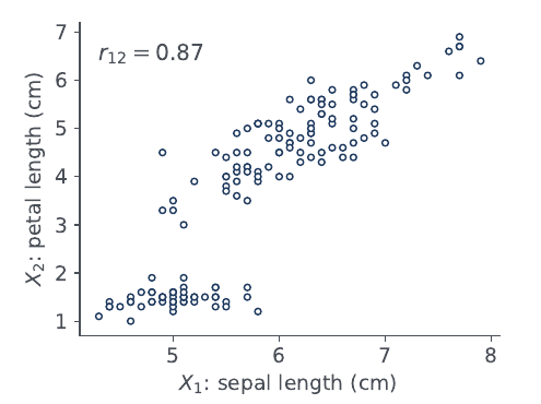
High correlation makes \(\bar D^T \bar D\) nearly singular: its determinant \(ae - c^2\) is small, so the inverse has large entries and small changes in the data swing the weights a lot.
In software, and a warning about training error
Software does the whole fit in three lines. But a small error on the training data does not prove the model will predict well on new data.
The old model is a special case of the new one (set the new weight to 0). Least squares picks the best of a bigger set, so it can only do at least as well. That is also why training error is a poor judge.
Part 6
Exam toolkit
Which formula, when
| The question asks for… | Use | Card |
|---|---|---|
| the line for one predictor, data given as a table | \(w = \dfrac{\sum (x_i-\mu_X)(y_i-\mu_Y)}{\sum (x_i-\mu_X)^2}\), then \(b = \mu_Y - w\mu_X\) | Slope & intercept |
| the line when only \(\sigma_{XY}\), \(\sigma_X^2\) and the means are given | \(w = \sigma_{XY}/\sigma_X^2\), \(b = \mu_Y - w\mu_X\) | Slope & intercept |
| “the geometric approach” or “the normal equations” | \(A = [\mathbf 1 \; X]\), \((b,w)^T = (A^T A)^{-1} A^T Y\), \(\hat Y = A(b,w)^T\) | Projection view |
| two or more predictors by hand | centre, \(\mathbf w = (\bar D^T \bar D)^{-1} \bar D^T \bar Y\), \(b = \mu_Y - \mathbf w^T \boldsymbol\mu_X\) | Hand calculation (centred) |
| a prediction for a new input | \(\hat y = b + \mathbf w^T \mathbf x\); flag extrapolation if \(\mathbf x\) is outside the data range | Linear model |
| the residuals, SSE, or a check of the fit | \(\epsilon_i = y_i - \hat y_i\), \(\mathrm{SSE} = \sum \epsilon_i^2\), confirm \(\sum \epsilon_i = 0\) and \(\sum x_i \epsilon_i = 0\) | Residuals |
| a typical error size in the units of \(Y\) | \(\mathrm{RMSE} = \sqrt{\mathrm{SSE}/n}\) | RMSE |
| whether a straight line is adequate | look at the residual plot, not just the SSE | Residual plots |
| why a weight changed after adding a predictor | correlated predictors share the credit | Correlated predictors |
- Show every step: the sums table, the determinant, the inverse, then the weights.
- Check the mean point: the fitted line must pass through \((\mu_X, \mu_Y)\). If it does not, something is wrong.
- Matrix multiplication: for \((A^T A)^{-1} A^T Y\), compute \(A^T Y\) first (a small vector), then multiply by the inverse.