Discrete random variables
The first half of Lecture 4 (binomial, multinomial, Poisson) and Part 1 of Lecture 5 (random variables, pmf and cdf, Bernoulli, geometric, expected value, variance, skewness), rebuilt as one storyline: turn outcomes into numbers, describe how the numbers are distributed, then recognise the four named distributions by what they count.
How to read this page. It needs the probability rules from Design, probability and Bayes, in particular counting. The continuous story continues on The normal curve and the CLT.
Teal = explanation added by Claude, not on the slides. Amber = watch out. Dropdowns hide worked examples, practice questions, and their answers.
The road through the lectures
Side stop: the multinomial distribution (L4 s11), which the exam toolkit mentions but no assignment has used.
Lecture map: which slides each card covers
Part 1
Random variables and their distributions
What a pmf and a cdf are, and the two numbers (mean, variance) plus one shape number (skewness) that summarise them.
Random variables and probability distributions
A random variable is a rule that attaches a number to each outcome of an experiment, such as "the number of yes answers". Its distribution is the list of the values it can take and how likely each one is.
- \(X, Y\)
- random variables
- \(x, y, k\)
- a particular value
- support
- the set of values the variable can take (e.g. \(0, 1, \dots, n\))
On page 1 the capital letter was a column of data you had not looked at yet. Here it is the same idea one step earlier: a quantity the experiment has not produced yet, with a known recipe for its probabilities.
The probability mass function (pmf)
The pmf gives the probability of each exact value. Every entry sits between 0 and 1, and the entries add up to 1, which is your check that a distribution is complete.
The sausage probabilities on L3 s65 add to 0.44, not 1, so as written they are not a complete distribution (the remaining 0.56 would belong to other counts). Always add up the column: if it is not 1, something is missing or wrong.
The cumulative distribution function (cdf): at most, at least, exactly
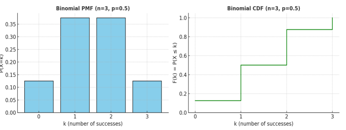
The cdf at a value is the probability of landing at or below it, so it is the pmf added up from the left. "At most k" is the cdf; "at least k" is one minus the cdf just below k; "exactly k" is the pmf.
| Phrase | Symbol | Values that count (out of 0–5) | Compute |
|---|---|---|---|
| at least 2, no fewer than 2 | \(X \ge 2\) | 2, 3, 4, 5 | \(1 - F(1)\) |
| at most 2, no more than 2 | \(X \le 2\) | 0, 1, 2 | \(F(2)\) |
| more than 2 | \(X \gt 2\) | 3, 4, 5 | \(1 - F(2)\) |
| fewer than 2, less than 2 | \(X \lt 2\) | 0, 1 | \(F(1)\) |
| exactly 2 | \(X = 2\) | 2 | \(P(2) = F(2) - F(1)\) |
| between 1 and 3 inclusive | \(1 \le X \le 3\) | 1, 2, 3 | \(F(3) - F(0)\) |
Does the boundary count? "At least" and "at most" include it; "more than" and "fewer than" exclude it. Before calculating, list the possible values and circle the ones the question allows.
"At least 2" and "at most 2" are not complements; both contain 2. The complement of "at least 2" is "at most 1". And the one-step shift (\(X \gt 2\) is the same as \(X \ge 3\)) works only for integer counts, not for continuous measurements.
X = absences from a group of four: write the inequality and allowed values for six phrases
At least 3 · at most 1 · more than 1 · fewer than 3 · exactly 2 · no more than 2.
\(X \ge 3\): 3, 4. \(X \le 1\): 0, 1. \(X \gt 1\): 2, 3, 4. \(X \lt 3\): 0, 1, 2. \(X = 2\): 2. \(X \le 2\): 0, 1, 2. These identify the events; the probabilities need the experiment.
Requests X with P = 0.10, 0.25, 0.35, 0.20, 0.10 for x = 0…4: at least 2, more than 2, at most 2, between 1 and 3
- \[ P(X \ge 2) = 0.35 + 0.20 + 0.10 = 0.65 = 1 - (0.10 + 0.25) \]
- \[ P(X \gt 2) = 0.20 + 0.10 = 0.30 \] (the 0.35 difference is the boundary value \(X = 2\))
- \[ P(X \le 2) = 0.10 + 0.25 + 0.35 = 0.70 \]
- \[ P(1 \le X \le 3) = 0.25 + 0.35 + 0.20 = 0.80 \]
Reward X = 0, 2, 5 QAR with probabilities 0.5, 0.3, 0.2: F(2) and P(2 < X ≤ 5)
- \[ F(2) = 0.5 + 0.3 = 0.8 \]
- \[ P(2 \lt X \le 5) = F(5) - F(2) = 1 - 0.8 = 0.2 \] Only the value 5 is above 2 and at most 5.
Expected value, variance and standard deviation of a random variable
The expected value is the long-run average you would see over many repeats: each value weighted by its probability. The variance is the probability-weighted average squared distance from that mean, and the standard deviation its square root.
- \(E[X],\ \mu\)
- expected value (mean) of the distribution
- \(E[X^2]\)
- \(\sum x_i^2 P(x_i)\); gives the shortcut \(\text{Var}(X) = E[X^2] - \mu^2\)
Computing \((x_i - \mu)^2\) for every value is tedious when \(\mu\) is a decimal. The same answer comes from \(\text{Var}(X) = E[X^2] - \mu^2\): square each value, weight by probability, subtract the squared mean. The L5 practice set answers (P3) use this route.
Recipe
- Table with a row \(x_i\) and a row \(P(x_i)\). Check the probabilities sum to 1.
- Row \(x_i P(x_i)\); its sum is \(\mu\).
- Row \(x_i^2 P(x_i)\); its sum is \(E[X^2]\).
- \[ \text{Var}(X) = E[X^2] - \mu^2,\qquad \sigma = \sqrt{\text{Var}(X)} \]
Daily service calls: P(0) = 0.3, P(1) = 0.4, P(2) = 0.2, P(3) = 0.1. E(X), Var(X), SD
- \[ E(X) = 0(0.3) + 1(0.4) + 2(0.2) + 3(0.1) = 1.1 \]
- \[ E(X^2) = 0 + 0.4 + 0.8 + 0.9 = 2.1 \]
- \[ \text{Var}(X) = 2.1 - 1.1^2 = 0.89 \]
- \[ \sigma = \sqrt{0.89} = 0.943 \text{ calls} \]
X = 0, 1, 2 with P = 0.5, 0.3, 0.2: E(X), Var(X), SD
- \[ E(X) = 0.3 + 0.4 = 0.7 \]
- \[ \text{Var}(X) = 0.49(0.5) + 0.09(0.3) + 1.69(0.2) = 0.61 \]
- \[ \sigma = 0.78 \]
Reward 0, 2, 5 QAR with P = 0.5, 0.3, 0.2; each play costs 2 QAR: E[X], the "impossible answer" objection, expected net gain
- \[ E[X] = 0(0.5) + 2(0.3) + 5(0.2) = 1.60 \text{ QAR} \]
- An expected value is a probability-weighted average, the long-run average over many plays. It need not be a possible single payout.
- \[ E[\text{net}] = 1.60 - 2 = -0.40 \text{ QAR per play} \]
Skewness: a number for the direction of the tail
Skewness measures how lopsided a distribution is. Zero means balanced tails, positive means a long tail to the right, negative a long tail to the left.
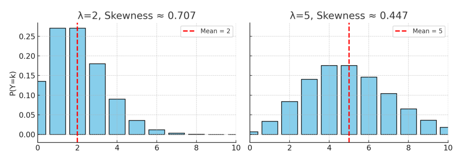
Bernoulli and binomial share the sign of \(1 - 2p\): the rarer outcome is in the tail. The geometric is never symmetric because it starts at 1 and stretches to infinity. The Poisson skewness only depends on \(\lambda\): doubling the interval doubles \(\lambda\) and shrinks the skewness by \(\sqrt 2\).
Y1 ~ Bernoulli(0.4), Y2 ~ Geometric(0.4), Y3 ~ Poisson(2): mean, SD, skewness; which is most symmetric; which model for a quality manager
- Bernoulli: \[ \mu = 0.4,\quad \sigma = \sqrt{0.24} = 0.490,\quad \gamma_1 = \frac{0.2}{0.490} = 0.408 \]
- Geometric: \[ \mu = \tfrac{1}{0.4} = 2.5,\quad \sigma = \sqrt{\tfrac{0.6}{0.16}} = \sqrt{3.75} = 1.936,\quad \gamma_1 = \frac{1.6}{\sqrt{0.6}} = 2.066 \]
- Poisson: \[ \mu = 2,\quad \sigma = \sqrt 2 = 1.414,\quad \gamma_1 = \tfrac{1}{\sqrt 2} = 0.707 \]
- Most symmetric: the Bernoulli (0.408), because \(p = 0.4\) is close to 0.5. The geometric is strongly right-skewed.
- For monitoring defects, the answer key picks Poisson: monitoring means counting defects per hour or shift, and \(\lambda\) gives control limits directly (e.g. \(\lambda + 3\sqrt\lambda = 6.2\)). Bernoulli describes one item; geometric the wait until the first defect.
Part 2
The named distributions
Bernoulli for one trial, binomial for a fixed number of trials, geometric for the wait until the first success, Poisson for counts per interval.
Bernoulli: one yes/no trial
A Bernoulli variable is a single trial coded 1 for success and 0 for failure. It is the building block: a binomial adds up many of them, a geometric counts how many you need until the first 1.
Indicator of a defective bulb, p = 0.2: pmf, E[X], Var(X), skewness
- \[ P(X = 1) = 0.2,\qquad P(X = 0) = 0.8 \]
- \[ E[X] = 0.2,\qquad \text{Var}(X) = 0.2 \times 0.8 = 0.16 \]
- \[ \gamma_1 = \frac{1 - 0.4}{\sqrt{0.16}} = \frac{0.6}{0.4} = 1.5 \] Right-skewed: the rare value 1 is the tail.
Binomial: successes in a fixed number of trials
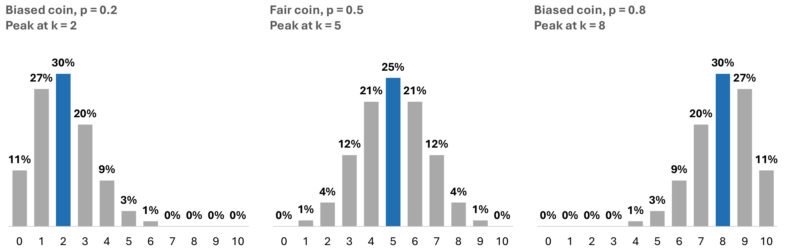
Flip a coin n times and count the heads: that count is binomial. The formula is "number of arrangements, times the chance that the k successes happen, times the chance that the other n − k fail".
- \(n\)
- number of trials (fixed in advance)
- \(p\)
- success probability, the same every trial
- \(k\)
- number of successes asked about, \(0 \le k \le n\)
Check the three conditions before using the formula: fixed \(n\), independent trials, constant \(p\). Drawing without replacement breaks independence (page 2, pens), so that is not binomial. And "success" is just the outcome being counted; a defective chip can be the "success".
Recipe
- Identify \(n\), \(p\), and what \(k\) the question wants (exactly, at most, at least).
- \[ \binom{n}{k} \] by cancelling factorials.
- \[ P(X = k) = \binom{n}{k} p^k (1-p)^{n-k} \]
- "At most \(k\)": add \(P(0)\) to \(P(k)\). "At least 1": \(1 - (1-p)^n\).
Chips 20% defective, test 5; and rainy days in a week with p = 0.3
- \[ P(X = 1) = 5 \times 0.2 \times 0.8^4 = 0.410 \]
- \[ P(X \ge 1) = 1 - 0.8^5 = 0.672 \]
- \[ E[X] = 5(0.2) = 1,\qquad \sigma = \sqrt{0.8} = 0.89 \]
- Rainy days, assuming independent days: \[ P(X = 2) = \binom{7}{2} 0.3^2\, 0.7^5 = 21 \times 0.09 \times 0.168 = 0.318 \]
Defectives independent with p = 0.05 in a batch of 20: P(exactly 2), P(at most 1)
- \[ P(X = 2) = \binom{20}{2}(0.05)^2(0.95)^{18} = 190 \times 0.0025 \times 0.3972 = 0.189 \]
- \[ P(X \le 1) = 0.95^{20} + 20(0.05)(0.95)^{19} = 0.358 + 0.377 = 0.736 \]
X ~ Binomial(12, 0.1): pmf, P(X ≤ 2), E[X], Var(X)
- \[ P(X = k) = \binom{12}{k}(0.1)^k(0.9)^{12-k} \]
- \[ P(0) = 0.9^{12} = 0.2824,\quad P(1) = 12(0.1)(0.9)^{11} = 0.3766,\quad P(2) = 66(0.01)(0.9)^{10} = 0.2301 \]
- \[ P(X \le 2) = 0.2824 + 0.3766 + 0.2301 = 0.889 \]
- \[ E[X] = 1.2,\qquad \text{Var}(X) = 12(0.1)(0.9) = 1.08,\qquad \sigma = 1.039 \]
Fair coin: P(exactly 6 heads in 10 flips); P(at least one head in 3 flips)
- \[ \binom{10}{6} \times 0.5^{10} = \frac{210}{1024} = 0.205 \]
- \[ P(X \ge 1) = 1 - P(X = 0) = 1 - 0.125 = 0.875 \]
Five transmissions, each succeeds with 0.20: name the model; P(X ≥ 1), E[X], Var(X)
- Binomial(5, 0.2): a fixed number of independent trials with the same success probability, counting successes.
- \[ P(X \ge 1) = 1 - 0.8^5 = 0.672 \]
- \[ E[X] = 1,\qquad \text{Var}(X) = 5(0.2)(0.8) = 0.8 \]
Multinomial: more than two outcomes per trial
When each trial can land in one of several categories instead of just success or failure, the binomial generalises to the multinomial. The counting factor becomes a factorial for every category.
The die example, computed
- \[ \frac{12!}{2!\,3!\,1!\,6!} = 55{,}440 \]
- Faces 4, 5, 6 together have probability \(\tfrac12\), so the probability factor is \(\left(\tfrac16\right)^{2+3+1}\left(\tfrac12\right)^6\).
- \[ P = 55{,}440 \times \left(\tfrac{1}{6}\right)^6 \left(\tfrac{1}{2}\right)^6 = 0.0186 \]
L4 s11 writes the probability factor as \((1/6)^{12}\), which treats "4, 5 or 6" as one face with probability 1/6. That gives \(2.5 \times 10^{-5}\), too small by a factor of \(3^6 = 729\). Grouped categories get the grouped probability.
Geometric: trials until the first success
Keep trying until the first success and count how many attempts it took. The first y − 1 attempts fail and the y-th succeeds, which gives the formula directly.
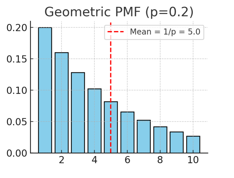
Past failures do not change the future: given that the first two attempts failed, the wait from now on is a fresh geometric. So "first success on attempt 4 given the first two failed" is just "attempt 3 fails and attempt 4 succeeds", \((1-p)\,p\). Dividing \(P(T = 4)\) by \(P(T \gt 2) = (1-p)^2\) gives the same thing.
Components tested until the first defective, p = 0.2: support, mean, variance, SD, skewness, shape
- \(X = 1, 2, 3, \dots\) with no upper limit. \(p = 0.2\) is the probability that any single component is defective.
- \[ \mu = \frac{1}{0.2} = 5 \] On average she tests 5 components to find the first defective one.
- \[ \sigma^2 = \frac{0.8}{0.04} = 20,\qquad \sigma = \sqrt{20} = 4.47 \]
- \[ \gamma = \frac{2 - 0.2}{\sqrt{0.8}} = \frac{1.8}{0.894} = 2.01 \]
- Positive, so right-skewed. The smallest value is 1 and there is no largest: most runs end after a few tests, but a long lucky streak of good components makes a long right tail.
Items fail with 0.1, inspected until the first failure: P(X = 4), P(X ≤ 3)
- \[ P(X = 4) = 0.9^3 \times 0.1 = 0.0729 \]
- \[ P(X \le 3) = 1 - 0.9^3 = 0.271 \]
p = 0.3: P(first basket on the 3rd attempt) and expected attempts; login p = 0.25: P(first success on the 4th try) and E(Y)
- \[ 0.7^2 \times 0.3 = 0.147,\qquad E(Y) = \tfrac{1}{0.3} = 3.33 \]
- \[ 0.75^3 \times 0.25 = 0.105,\qquad E(Y) = \tfrac{1}{0.25} = 4 \]
Transmissions until the first success, p = 0.2: given the first two failed, P(first success on attempt 4)?
- Geometric(0.2) on 1, 2, 3, …: it counts attempts up to and including the first success.
- Given two failures, attempt 3 must fail and attempt 4 succeed: \[ P(T = 4 \mid T \gt 2) = 0.8 \times 0.2 = 0.16 \]
- Check: \(P(T = 4)/P(T \gt 2) = 0.8^3(0.2)/0.8^2 = 0.16\). Multiplying by the first two failures again would answer the unconditional question.
Poisson: events in a fixed interval of time or space
When events arrive at a steady average rate and independently of each other, the number in a fixed stretch of time or space is Poisson. One number, the average rate, fixes the whole distribution, and the count has no upper limit.
- \(\lambda\)
- average number of events per interval; scale it with the interval length
- \(e^{-\lambda}\)
- the probability of zero events; every other term is built on it
Match \(\lambda\) to the interval in the question. Three per hour is \(\lambda = 1\) for a 20-minute gap and \(\lambda = 6\) for two hours. L4 s45 prints the formula as \(e^{-v}\lambda^k/k!\); the exponent is \(-\lambda\).
Recipe
- Rescale \(\lambda\) to the interval asked about.
- \[ e^{-\lambda} \] once; keep it.
- \[ P(X = k) = e^{-\lambda}\,\frac{\lambda^k}{k!} \] for each \(k\) needed; "at most" adds them, "at least" uses the complement.
1.5 typos per page: P(none), P(at least two)
- \[ P(X = 0) = e^{-1.5} = 0.223 \]
- \[ P(X \ge 2) = 1 - e^{-1.5}(1 + 1.5) = 1 - 0.558 = 0.442 \]
Emails at 3 per hour: P(exactly 5 in an hour), P(none in a 20-minute gap), P(no calls in an hour)
- \[ P(X = 5) = \frac{e^{-3}\,3^5}{5!} = 0.101 \]
- Twenty minutes is a third of an hour, so \(\lambda = 1\): \[ P(X = 0) = e^{-1} = 0.368 \]
- No calls in an hour at \(\lambda = 3\): \[ e^{-3} = 0.050 \]
Café arrivals λ = 4 per 10 minutes: E[Y], σ, skewness; P(exactly 5)
- \[ E[Y] = 4,\qquad \sigma = 2,\qquad \gamma_1 = \tfrac{1}{2} = 0.5 \] (mildly right-skewed)
- \[ P(Y = 5) = \frac{e^{-4}\,4^5}{5!} = \frac{0.01832 \times 1024}{120} = 0.156 \]
Requests at 6 per hour; N = count in 20 minutes: P(N ≤ 1); is the 60-minute count more or less skewed?
- \[ \lambda = 6 \times \tfrac{20}{60} = 2 \]
- \[ P(N \le 1) = e^{-2} + 2e^{-2} = 3e^{-2} = 0.406 \]
- For 60 minutes \(\lambda = 6\): skewness \(1/\sqrt 6 = 0.408\) against \(1/\sqrt 2 = 0.707\). Less right-skewed, although its mean and variance are larger.
Choosing a discrete model: read what X counts
Before touching a formula, say in words what the random variable counts. One trial, successes out of a fixed n, attempts until the first success, or events per interval: each phrase names its distribution.
Name the model: defectives in a batch of 20; typos per page; login attempts until the first success
(a) binomial, (b) Poisson, (c) geometric.
A single flip, a few flips, many flips: which description fits each?
A single flip: a single probability (Bernoulli). A few flips: the binomial distribution, a pmf. Many flips: the normal distribution, a pdf, which is where the next page starts.
Part 3
Exam toolkit
Formulas for mean, variance and skewness are usually given; the mark is for choosing and applying them.
Which formula, when
| The question asks for… | Use | Card |
|---|---|---|
| "exactly k" | the pmf \(P(X = k)\) | pmf |
| "at most k" | \(F(k) = \sum_{i \le k} P(i)\) | cdf |
| "at least k" | \(1 - F(k-1)\); for "at least 1", \(1 - P(0)\) | cdf |
| long-run average of a table | \(E[X] = \sum x\,P(x)\) | E(X) |
| spread of a table | \(\text{Var} = \sum x^2 P(x) - \mu^2\) | Var(X) |
| which way the tail points | sign of \(\gamma_1\) | Skewness |
| one yes/no trial | \(p\), \(p(1-p)\), \((1-2p)/\sqrt{p(1-p)}\) | Bernoulli |
| k successes out of n | \(\binom{n}{k}p^k(1-p)^{n-k}\); \(np\); \(np(1-p)\) | Binomial |
| first success on trial k | \((1-p)^{k-1}p\); \(1/p\); \((1-p)/p^2\); \(F(k) = 1 - (1-p)^k\) | Geometric |
| k events per interval | \(e^{-\lambda}\lambda^k/k!\); mean and variance \(\lambda\); rescale \(\lambda\) to the interval | Poisson |
| counts in several categories | \(\frac{n!}{x_1!\cdots x_k!}p_1^{x_1}\cdots p_k^{x_k}\) | Multinomial |
| which model | what does X count? | Which model |