The normal curve, z-scores and the central limit theorem
Parts 2 to 6 of Lecture 5 (slides 41–130), rebuilt as one storyline: where the bell curve comes from, how one table answers every normal-probability question, why averages of anything become normal, and what changes when the variables are dependent.
How to read this page. It needs the binomial and the expected value from Discrete random variables. The midterm covered the normal density but not the z-table or the CLT; the final will.
Teal = explanation added by Claude, not on the slides. Amber = watch out. Dropdowns hide worked examples, practice questions, and their answers.
The road through the lecture
Side stops: critical values, anecdotes vs distributions, Poisson planning, and two continuous models (uniform, exponential) that appear only on the practice sheets.
Lecture map: which slides each card covers
Part 1
Where the bell curve comes from
Repeated coin flips to the normal density, one piece of the formula at a time.
From the binomial to a bell
Flip a fair coin forty times and the most likely count is twenty heads, with the probabilities falling away symmetrically on both sides in a bell shape. Average many such experiments and the averages form the same bell.
The slides show two things. First, the binomial itself looks bell-shaped once \(n\) is large. Second, the average of many repetitions is bell-shaped. The second is the central limit theorem in Part 4, and it holds for averages of almost anything, not only coins.
The normal density, built step by step
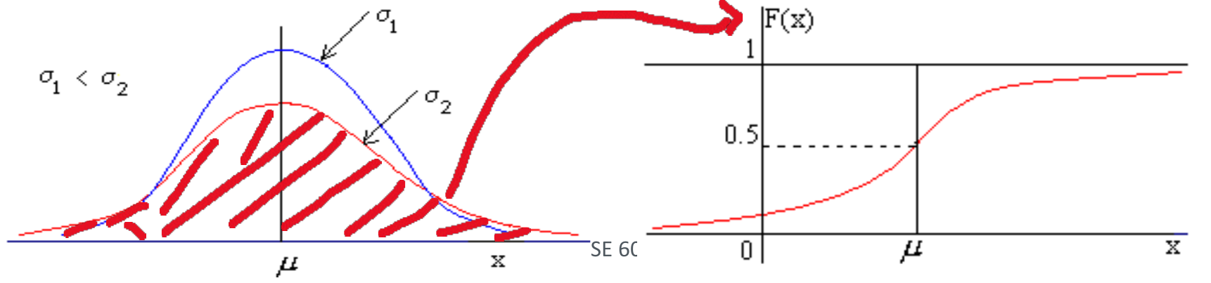
The bell curve is an exponential of a downward parabola. The parabola is centred at the mean, its width is set by the variance, the minus sign makes the curve fall away on both sides, and a constant in front makes the total area one.
- \(\mu\)
- centre: the peak, which is also the median and the mode
- \(\sigma\)
- width: larger \(\sigma\) gives a lower, wider curve
- \(1/\sqrt{2\pi\sigma^2}\)
- the peak height; it makes the total area 1
- \(X \sim N(\mu, \sigma^2)\)
- "\(X\) is normal with mean \(\mu\) and variance \(\sigma^2\)"
The second parameter in \(N(\mu, \sigma^2)\) is the variance. \(N(500, 40^2)\) has standard deviation 40, not 1600. Before standardising, check whether the question hands you \(\sigma\) or \(\sigma^2\).
Where is the density largest; what happens when σ doubles; could a plus sign in the exponent give a density?
- At \(x = \mu\): the squared deviation is zero there, so the exponent reaches its maximum of zero and the exponential equals 1. Everywhere else the exponent is negative.
- Doubling \(\sigma\) doubles the horizontal scale (wider curve) and halves the peak height \(1/(\sigma\sqrt{2\pi})\). The area stays 1.
- No. A positive exponent grows as \(|x - \mu|\) grows, so the integral over the real line is infinite and no constant can normalise it to 1.
Part 2
The standard normal and z-scores
Convert any normal value to a z-score, read the table, translate the words into an area.
Why the normal matters, and the 68–95–99.7 rule
About two thirds of a normal variable's values lie within one standard deviation of the mean, 95 percent within two, and almost all within three. That rule works for any mean and any standard deviation.
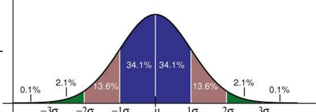
From the figure, \(P(Z \gt 2) = 2.1\% + 0.1\% = 2.2\%\), close to the table's 2.28%. The bands are a fast sanity check for any z-table answer.
The z-score: distance from the mean in standard deviations
A z-score says how many standard deviations a value sits above or below its mean. It lets you compare scores from different scales, and it is the key that opens the standard normal table.
Mean 100, SD 20: the z-score of 140?
\(z = (140 - 100)/20 = 2\).
Reading the standard normal table: below, above, between
The table gives the area to the left of a z-score, which is the probability of being below it. "Above" is one minus that, "between" is the difference of two lookups, and you should always draw and shade the curve before looking anything up.
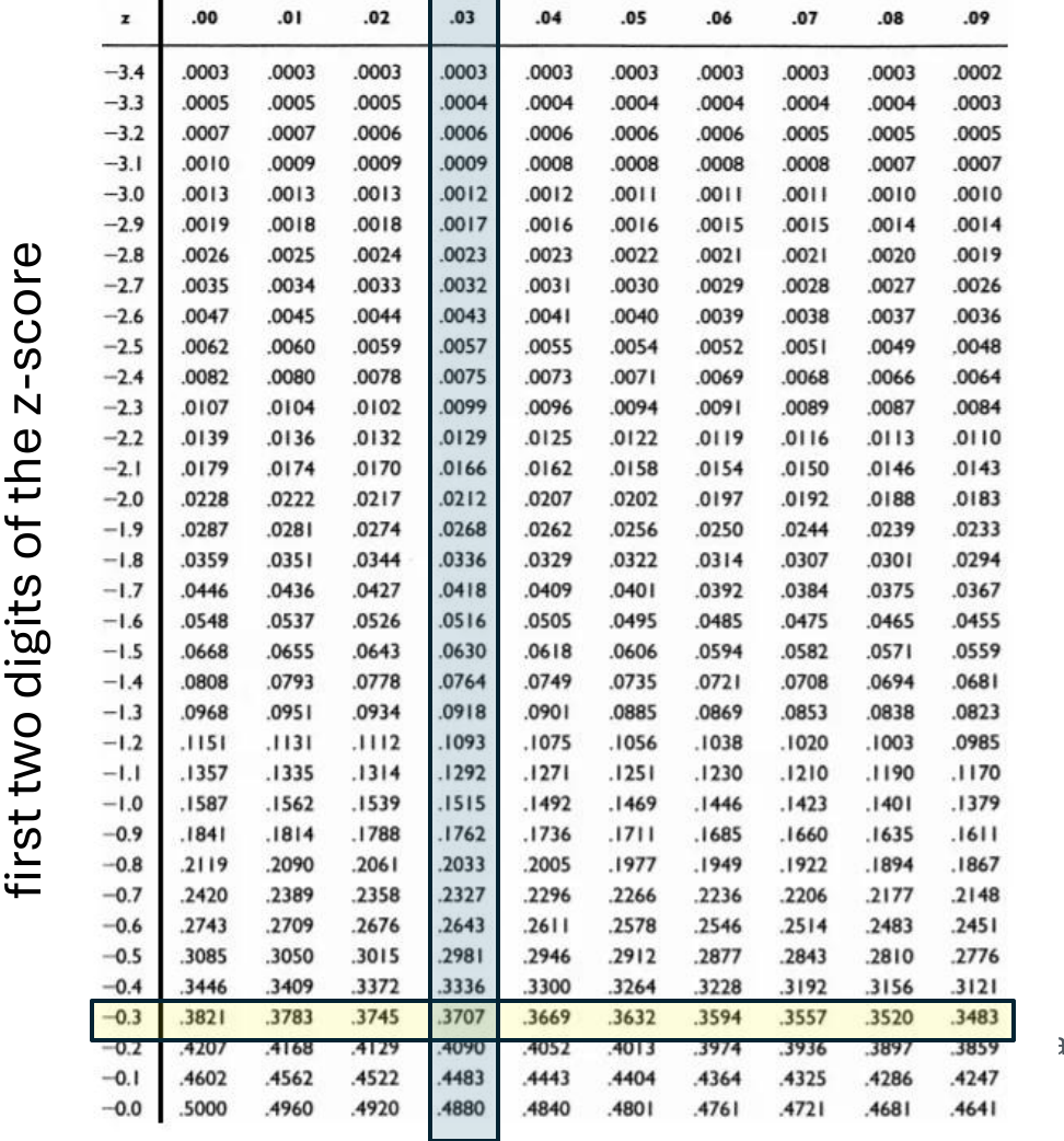
Some tables list the area to the left, some the area between 0 and \(z\), some the upper tail. Check the picture at the top of the table before reading a number. For a continuous variable \(P(X \le a) = P(X \lt a)\): the boundary carries no probability.
Recipe
- Sketch and shade.
- \[ z = \frac{x - \mu}{\sigma} \] for each boundary.
- Look up \(\Phi(z)\) for each.
- Below: \(\Phi\). Above: \(1 - \Phi\). Between: difference.
- Sanity check against the empirical rule.
Bulb lifetimes N(1200, 100²): P(more than 1350 hours)
- \[ z = \frac{1350 - 1200}{100} = 1.5 \]
- \[ P = 1 - \Phi(1.5) = 1 - 0.9332 = 0.0668 \] About one bulb in fifteen.
Birth weights N(3300, 500²): P(2800 < X < 4000); the weight exceeded by only 5%
- \[ z_{2800} = -1.0,\qquad z_{4000} = 1.4 \]
- \[ P = \Phi(1.4) - \Phi(-1.0) = 0.9192 - 0.1587 = 0.760 \]
- Top 5%: the z with 95% below it is 1.645 (see critical values).
- \[ x = 3300 + 1.645 \times 500 = 4123 \text{ g} \]
Scores N(500, 100²): P(above 636), P(above 233), P(above 815)
- \[ z = 1.36:\quad 1 - \Phi(1.36) = 1 - 0.9131 = 0.0869 \]
- \[ z = -2.67:\quad 1 - \Phi(-2.67) = 1 - 0.0038 = 0.9962 \]
- \[ z = 3.15:\quad 1 - \Phi(3.15) = 1 - 0.9992 = 0.0008 \]
Critical values of the standard normal
A critical value is the table read backwards: given a tail area, which z cuts it off? Three of them come up constantly and are worth memorising.
"Exceeded by only 5%" is one tail: \(z = 1.645\). "The middle 95%" is two tails of 2.5% each: \(z = \pm 1.96\). Say which one the question is before picking the number.
Part 3
Distributions in practice
Anecdote versus aggregate evidence, and a Poisson stock-level decision.
The counterexample method and why distributions matter
One ninety-year-old smoker does not disprove that smoking shortens life, because the claim is about averages, not about every person. A single case can show something is possible, never that it is typical.
"My relative smoked 40 years and lived to 95, so smoking is not harmful." What is wrong?
One person is a single draw from a distribution with wide spread. Surviving to 95 has non-zero probability for smokers, so the case is consistent with smoking being harmful. The claim can only be tested on the whole distribution, where smokers have a lower mean lifetime and a much higher risk of early death.
From probability to planning: catering with a Poisson model
To decide how many meals to prepare, you need the chance that attendance is at most your capacity, which is the cumulative probability, not the chance of hitting the capacity exactly. A buffer of ten percent over the mean turns out to be far more than enough when the mean is in the thousands.
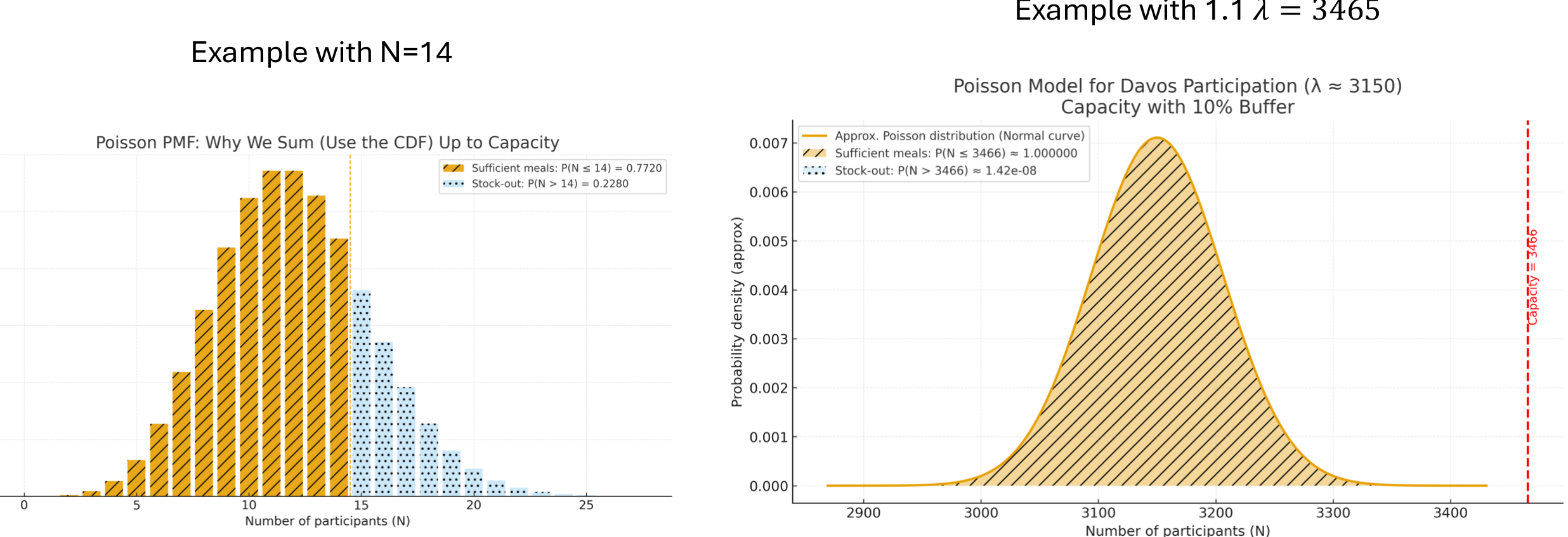
A 10% buffer is \(315\) meals, and the SD is only 56, so the capacity is \(z = 315/56 = 5.6\) standard deviations above the mean. For a Poisson with a large \(\lambda\) the normal approximation is excellent, and \(1 - \Phi(5.6)\) is about \(10^{-8}\). The size of the buffer should be set in standard deviations, not percent.
Weekly demand Poisson(4): how many units so that demand is met in at least 95% of weeks?
- \[ P(X \le 7) = 0.949,\qquad P(X \le 8) = 0.979 \]
- Stock 8 units. Stocking 7 leaves a 5.1% stock-out risk, just above the 5% limit.
Part 4
Sampling distributions and the central limit theorem
A statistic varies from sample to sample. The CLT says how.
Sampling distributions
Take a sample, compute a statistic, repeat: the statistic comes out different each time. The pattern of those values is the sampling distribution, and it tells you how far your one estimate is likely to be from the truth.
As the sample size grows, the sample mean (or proportion) gets closer and closer to the population mean (or proportion). The CLT adds how it is spread around that target on the way there.
The central limit theorem: statement, conditions, mean and variance of the sample mean
Average enough independent draws from any distribution and the average is approximately normal, centred on the population mean, with a spread that shrinks like one over the square root of the sample size. The original data need not be normal at all.
- \(\bar X_n\)
- the mean of a sample of size \(n\), a random variable
- \(\sigma/\sqrt n\)
- standard error (SE): the SD of the sample mean
- i.i.d.
- independent and identically distributed
The theorem is about the sample mean, not the individual observations. Dividing \(\sigma\) by \(\sqrt n\) is the step students skip most often; and it is the square root of \(n\), not \(n\).
Give an example where a normal approximation to the binomial is appropriate
Any binomial with large \(n\) and \(p\) not too close to 0 or 1, so that \(np\) and \(n(1-p)\) are both at least about 10: for example the number of heads in 100 fair flips, \(X \sim \text{Binomial}(100, 0.5)\), approximately \(N(50, 25)\). The ten-flip picture on the previous page already looks bell-shaped; a hundred flips is close to a perfect bell.
Probabilities for a sample mean
To get the chance that an average exceeds some value, standardise with the standard error instead of the standard deviation, then use the z-table exactly as before.
L5 s106 reads the table as 0.994 and reports \(1 - 0.994 = 0.006\). The table value for \(z = 3.25\) is 0.9994, so the tail is 0.0006, ten times smaller. (The slide's "between" calculation on s108 uses the correct 0.9994.) Also, with \(n = 4\) and no statement that weights are normal, the CLT is being stretched; the slide assumes it anyway.
Recipe
- Identify \(\mu\), \(\sigma\), \(n\), and the value of the mean asked about.
- \[ \text{SE} = \frac{\sigma}{\sqrt n} \]
- \[ z = \frac{\bar x - \mu}{\text{SE}} \]
- Below, above or between with the table.
μ = 50, σ = 10, n = 25, P(mean > 52); and bulbs μ = 1000, σ = 200, n = 64
- \[ \text{SE} = \frac{10}{5} = 2,\qquad z = \frac{52 - 50}{2} = 1 \]
- \[ P(\bar X \gt 52) = 1 - 0.8413 = 0.1587 \]
- Bulbs: \[ \text{SE} = \frac{200}{8} = 25 \]
- \[ P(\bar X \lt 950):\quad z = -2,\quad \Phi(-2) = 0.0228 \]
- \[ P(980 \lt \bar X \lt 1020):\quad z = \pm 0.8,\quad 0.7881 - 0.2119 = 0.576 \]
μ = 70, σ = 12, n = 36: P(sample mean > 73)
- \[ \text{SE} = \frac{12}{6} = 2,\qquad z = \frac{73 - 70}{2} = 1.5 \]
- \[ P = 1 - 0.9332 = 0.0668 \]
Dog weights μ = 25 kg, σ = 6; n = 100: P(24 < sample mean < 26)
- \[ \text{SE} = \frac{6}{10} = 0.6,\qquad z = \pm\frac{1}{0.6} = \pm 1.67 \]
- \[ P = \Phi(1.67) - \Phi(-1.67) = 0.9525 - 0.0475 = 0.905 \]
20% of components fail; in a sample of 400, P(more than 24% fail)
- A proportion is a mean of 0/1 values, so the same theorem applies with \(\sigma^2 = p(1-p)\):
- \[ \text{SE} = \sqrt{\frac{0.2 \times 0.8}{400}} = 0.02 \]
- \[ z = \frac{0.24 - 0.20}{0.02} = 2.0,\qquad P = 1 - 0.9772 = 0.0228 \]
The proportion formula is not on the slides; it follows from the Bernoulli variance on the previous page.
Part 5
Dependent variables and covariance
When the variables move together, variances no longer simply add.
Variance and SD of a sum of dependent variables
The variance of a sum is the sum of the variances plus twice the covariance. If the variables rise and fall together the covariance is positive and the sum is more variable than independence would suggest.
With \(\text{Cov} = 0\) the formula collapses to \(\text{Var}(X) + \text{Var}(Y)\), which is what the CLT proof on the previous card used. A negative covariance (a hedge) makes the sum less variable than either part.
Sampling distribution of the mean when observations are dependent
If the observations in a sample are correlated, the sample mean is more variable than the formula sigma over root n says. Positive covariance between observations inflates the standard error.
Ignoring the covariances, \(\text{Var}(\bar X)\) would be \(15/9 = 1.67\) and SE 1.29. The three positive covariances add \(9/9 = 1\) to the variance. This is the "independence" limitation of the CLT in numbers.
Estimating covariance from paired data
Covariance measures whether two variables tend to be above their means at the same time. Multiply the two deviations for each pair, add up, and divide by n minus one.
Divide the covariance by the two standard deviations and you get Pearson's \(r\) from page 2: \(r = \text{Cov}(X, Y)/(s_X s_Y)\). Covariance has units (score × score) and no fixed scale; \(r\) is unit-free and lives in \([-1, 1]\).
Recipe
- Means of \(X\) and \(Y\).
- Deviation of each \(x\), each \(y\); their product per pair.
- \[ \text{Cov} = \frac{\sum (x_i - \bar x)(y_i - \bar y)}{n-1} \]
X = 2, 4, 6, 8 and Y = 3, 7, 5, 11: sample covariance, then Var(X + Y)
- \[ \bar x = 5,\qquad \bar y = 6.5 \]
- Deviations \(x\): −3, −1, 1, 3; \(y\): −3.5, 0.5, −1.5, 4.5. Products 10.5, −0.5, −1.5, 13.5; sum 22.
- \[ \text{Cov} = \frac{22}{3} = 7.33 \]
- \[ s_x^2 = \frac{20}{3} = 6.67,\qquad s_y^2 = \frac{35}{3} = 11.67 \]
- \[ \text{Var}(X + Y) = 6.67 + 11.67 + 2(7.33) = 33.0 \]
- Check directly: \(X + Y = 5, 11, 11, 19\), mean 11.5, sample variance \((42.25 + 0.25 + 0.25 + 56.25)/3 = 33.0\) ✓
Part 6
Side topics from the practice sheets
Two continuous models the slides do not cover but the instructor's practice sheets ask about.
Uniform and exponential distributions
A uniform variable is equally likely anywhere in an interval, so probabilities are just lengths. An exponential variable is a waiting time with a constant rate, the continuous cousin of the geometric.
If events are Poisson with rate \(\lambda\), the gap between events is exponential with mean \(1/\lambda\).
Shuttle wait uniform on [0, 20] minutes: pdf, mean, SD, P(5 < X < 12)
- Total area 1, so \(20h = 1\): \[ f(x) = \tfrac{1}{20} = 0.05 \text{ for } 0 \le x \le 20 \]
- \[ \mu = 10,\qquad \sigma^2 = \frac{400}{12} = 33.33,\qquad \sigma = 5.77 \]
- \[ P(5 \lt X \lt 12) = \frac{7}{20} = 0.35 \]
Sensor lifetime exponential with mean 200 hours: P(lasts at least 250); the median lifetime
- \[ \lambda = \tfrac{1}{200} \]
- \[ P(X \ge 250) = e^{-250/200} = e^{-1.25} = 0.287 \]
- \[ \text{median} = 200\ln 2 = 138.6 \text{ hours} \] (below the mean, because the distribution is right-skewed)
Midterm practice Q21 (a confidence interval for a proportion) belongs to the post-midterm material and is not covered here.
Part 7
Exam toolkit
Which formula, when
| The question asks for… | Use | Card |
|---|---|---|
| the peak, width or area of the bell | \(\mu\), \(\sigma\), \(1/\sqrt{2\pi\sigma^2}\) | Normal density |
| a rough share within 1, 2, 3 SD | 68%, 95%, 99.7% | Empirical rule |
| compare values on different scales | \(z = (x - \mu)/\sigma\) | z-score |
| P(below / above / between) | \(\Phi(z)\), \(1 - \Phi(z)\), \(\Phi(z_b) - \Phi(z_a)\) | z-table |
| the value cut off by a tail area | \(x = \mu + z_\alpha\sigma\), with 1.645 / 1.96 / 2.576 | Critical values |
| stock level for a service level | smallest \(C\) with Poisson cdf \(\ge\) target | Poisson planning |
| probability for a sample mean | SE \(= \sigma/\sqrt n\), then \(z = (\bar x - \mu)/\text{SE}\) | Sample mean |
| probability for a sample proportion | SE \(= \sqrt{p(1-p)/n}\) | Sample mean |
| variance of a sum | \(\text{Var}X + \text{Var}Y + 2\,\text{Cov}\) | Dependence |
| SE of a mean of correlated data | \(\frac1n\sqrt{\sum\text{Var} + 2\sum\text{Cov}}\) | Sampling with dependence |
| covariance from pairs | \(\sum(x_i-\bar x)(y_i-\bar y)/(n-1)\) | Covariance |
| equally likely over an interval | length / total length | Uniform |