Design, probability and Bayes
Lecture 3 (statistical inference, probability rules, conditional probability, Bayes) and the second half of Lecture 4 (slides 18–47, which revisit conditional probability and Bayes with tree diagrams), rebuilt as one storyline: from sample to population, then the rules for reasoning about chance, then how new evidence updates a probability.
How to read this page. It builds on Describing data and feeds the distributions on Discrete random variables. Every card says which slides it came from, what to read first, and what uses it later.
Teal = explanation added by Claude, not on the slides. Amber = watch out. Dropdowns hide worked examples, practice questions, and their answers.
The road through the lectures
Side stops: correlation (needed later for regression), the symbol table, and Warner's randomised-response survey.
Lecture map: which slides each card covers
Part 1
From sample to population
The vocabulary of inference and study design. Mostly definition questions in the exam.
Statistical science: population, sample, parameter, statistic
Statistics uses a sample you can see to learn about a population you cannot. A parameter is a number describing the whole population; a statistic is the same recipe applied to the sample, and it is our estimate of the parameter.
- \(\mu,\ \sigma,\ p\)
- population mean, SD, proportion: parameters, fixed and usually unknown
- \(\bar x,\ s,\ \hat p\)
- sample mean, SD, proportion: statistics, vary from sample to sample
Ask "whose number is it?" If it describes every subject of interest, it is a parameter. If it was computed from the subjects actually measured, it is a statistic. The same word "mean" can be either.
A company samples 50 employees per department. The 50 marketing scores represent a…
(a) population, (b) sample, (c) parameter, (d) statistic.
(b) sample: a subset of all marketing employees. Their average would be a statistic; the average over all marketing employees would be the parameter.
Explain parameter vs statistic with an example; is 62% in a poll of 1,200 a parameter?
A parameter is a fixed numerical summary of the whole population; a statistic is computed from a sample and changes from sample to sample. For the ten days of campus traffic (page 1): the mean traffic over all days of the year is a parameter \(\mu\); the sample mean of the ten recorded days, \(\bar x = 481\), is a statistic that estimates it. In the poll, 62% is \(\hat p\), a statistic; the share of all residents, \(p\), is the unknown parameter.
Study design: observe or intervene?
In an observational study you only watch what happens; in an experiment you assign the treatment yourself. Only the experiment can show cause and effect, because random assignment removes the other explanations.
Random assignment fixes causation (the groups differ only by the treatment). Random sampling fixes generalisation (the sample looks like the population). One does not buy you the other: a perfectly randomised experiment on volunteers still only tells you about people like the volunteers.
Experiment or observational study? Office hours and grades; new fertiliser; two checkout designs; parks and obesity
- (a) Observational: you cannot assign students to attend office hours; use existing attendance and grade data (explorative).
- (b) Experiment: assign plots to the new or the standard fertiliser and compare yield; this is the only way to attribute the difference to the fertiliser.
- (c) Experiment: an A/B test randomly shows each visitor design A or B and compares completion rates.
- (d) Observational: cities already have their parks; compare obesity rates across them (explanatory), remembering other city differences could explain the pattern.
Students randomly assigned to Method A or B and compared: what kind of study?
(b) Experiment. The researcher assigns the treatment (the method).
App users score 8 points higher: why can't you conclude the app "increases" scores?
A university emails all students; of those who reply, 60 use a study app and 40 do not. Users average 8 points more.
- Observational: students chose whether to use the app. A plausible alternative: more motivated students both adopt the app and score higher.
- Problem 1, causation: the groups may differ in motivation, ability or study time. Fix: randomly assign app access to comparable groups.
- Problem 2, generalisation: voluntary repliers need not represent all students. Fix: a representative random sample with effort to reduce non-response.
Explanatory, response, independent, dependent, control
The response is the outcome you are trying to explain, and the explanatory variables are the ones you use to explain it. These are roles chosen by your question, not labels stuck to the variables.
Describe two ways to pick a response variable among exercise, sleep, stress, diet, age, performance
Question 1: "what lifestyle factors affect academic performance?" Response: academic performance; explanatory: exercise, sleep, stress, diet, age. Question 2: "what influences stress?" Response: stress; explanatory: exercise, sleep, diet, age and academic performance. The research question decides the roles: whatever you want to predict is the response.
Experiment on whether fertiliser increases plant height: what is the response variable?
(b) Plant height: the outcome measured. Fertiliser amount is explanatory (independent); plant type and soil would be control variables.
Association vs correlation, and Pearson's r
Association means any kind of relationship between two variables. Correlation is one specific number, between −1 and +1, that measures how close two quantitative variables are to a straight line.
- \(\sum (x_i - \bar x)(y_i - \bar y)\)
- positive when \(x\) and \(y\) are above (or below) their means together
- \(\sum (x_i - \bar x)^2\)
- sum of squares of \(x\); its square root scales the numerator
\(r\) measures straight-line association only. A perfect U-shaped relationship can have \(r = 0\). And a strong \(r\) is not causation: a lurking variable can drive both (review p22 ex5).
Recipe
- Means \(\bar x\), \(\bar y\).
- Deviations of each \(x\) and each \(y\).
- \[ S_{xy} = \sum (x_i - \bar x)(y_i - \bar y) \]
- \[ S_{xx} = \sum (x_i - \bar x)^2,\qquad S_{yy} = \sum (y_i - \bar y)^2 \]
- \[ r = \frac{S_{xy}}{\sqrt{S_{xx} S_{yy}}} \]
Hours studied vs exam score for 7 students
- \(x = 1, 2, \dots, 7\); \(y = 50, 55, 60, 65, 70, 75, 85\).
- \[ \bar x = 4,\qquad \bar y = \frac{460}{7} = 65.71 \]
- \[ S_{xy} = 155,\qquad S_{xx} = 28,\qquad S_{yy} = 871.43 \]
- \[ r = \frac{155}{\sqrt{28 \times 871.43}} = 0.99 \]
- An almost perfect positive linear relationship: the points sit close to the trend line.
Compute \(r\) for \(x = 1,2,3,4,5\), \(y = 2,4,5,4,5\); then interpret \(r = -0.85\) between TV hours and GPA
- \[ \bar x = 3,\qquad \bar y = 4 \]
- Products of deviations: \((-2)(-2), (-1)(0), (0)(1), (1)(0), (2)(1)\) sum to 6.
- \[ S_{xx} = 10,\qquad S_{yy} = 6 \]
- \[ r = \frac{6}{\sqrt{60}} = 0.77 \]
- \(r = -0.85\): a strong negative linear association. It does not prove TV lowers GPA; a lurking variable (less study time, say) could drive both.
Symbol clarification
Roman letters are for the sample you measured, Greek letters for the population or the theoretical model. Same idea, different data.
Part 2
The rules of probability
Sample spaces, three axioms, and the complement, addition and multiplication rules every later formula is built from.
Two meanings of probability, and why statisticians need it
A probability is the fraction of times an outcome would happen if you repeated the experiment endlessly. People also use it for a degree of belief, the Bayesian reading, but this course mostly uses the first.
Sample space, events, complement, intersection, union
The sample space is the list of everything that could happen. An event is any part of that list, and "not A", "A and B", "A or B" are just ways of picking out other parts.
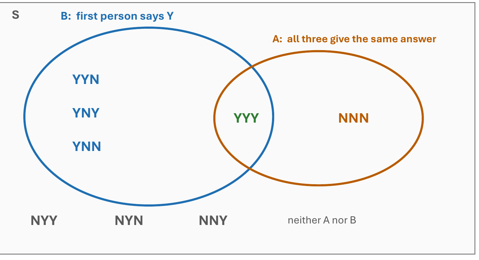
- \(A^c,\ \neg A\)
- not \(A\)
- \(A \cap B,\ AB,\ A \text{ and } B\)
- both happen
- \(A \cup B,\ A \text{ or } B\)
- at least one happens
Equally likely outcomes and the three axioms
When every outcome is equally likely, a probability is just counting: favourable outcomes over all outcomes. The three axioms say probabilities are never negative, the whole sample space has probability one, and probabilities of non-overlapping events add.
P(head) on one fair toss; P(defective) when 10 of 1,000 items are defective
- \[ P(H) = \frac{1}{2} \]
- \[ P(\text{defective}) = \frac{10}{1000} = 0.01 \] (not 0.001, and "0.1%" would be 0.001).
The complement rule and "at least one"
The chance that something does not happen is one minus the chance that it does. The trick to remember: "at least one" is the opposite of "none", so compute "none" and subtract from one.
At least one six in four rolls
- \[ P(\text{no six in 4 rolls}) = \left(\tfrac{5}{6}\right)^4 = 0.482 \]
- \[ P(\text{at least one six}) = 1 - 0.482 = 0.518 \]
One die: P(at least 4), P(more than 4), P(at most 4), P(fewer than 4), and the complement check
- At least 4: faces 4, 5, 6, so \(3/6 = 1/2\).
- More than 4: faces 5, 6, so \(2/6 = 1/3\).
- At most 4: faces 1 to 4, so \(4/6 = 2/3\).
- Fewer than 4: faces 1, 2, 3, so \(1/2\).
- The opposite of "at least 4" is "fewer than 4": \(1 - 3/6 = 1/2\) ✓. "At least 4" and "at most 4" are not opposites; both include 4.
Mutually exclusive events and the addition rule
To get the chance of "A or B", add the two chances, then take away the overlap so it is not counted twice. If the two events cannot happen together, there is no overlap to remove.
Recipe: "A or B" from a table
- Make a two-way table and fill in the totals.
- \[ P(A) + P(B) \]
- Subtract the cell that is in both.
Parent or female at a school-board meeting
- 9 parents (5 female, 4 male) and 5 teachers (2 female, 3 male): 14 people, 7 female.
- \[ P(\text{parent}) + P(\text{female}) = \tfrac{9}{14} + \tfrac{7}{14} = \tfrac{16}{14} \]
- \[ \tfrac{16}{14} - \tfrac{5}{14} = \tfrac{11}{14} \] Without the subtraction the 5 female parents are counted twice (and the answer exceeds 1).
Neither red nor blond hair; three or more children
- 43 students: brown 15, black 10, blond 16, red 2. "Neither red nor blond" means brown or black:
- \[ \tfrac{15}{43} + \tfrac{10}{43} = \tfrac{25}{43} = 0.581 \]
- Families: 4% have three children, 2% four or more. Three or more:
- \[ 0.04 + 0.02 = 0.06 \]
100 students: 30 in maths, 70 in physics, 20 in neither. P(maths), P(physics), P(either), P(both)? And 60% maths, 40% physics, 25% both.
- \[ P(M) = 0.30,\qquad P(Ph) = 0.70 \]
- \[ P(M \cup Ph) = 1 - P(\text{neither}) = 1 - 0.20 = 0.80 \]
- \[ P(M \cap Ph) = P(M) + P(Ph) - P(M \cup Ph) = 0.30 + 0.70 - 0.80 = 0.20 \]
- Review version: \(P(M \cup P) = 0.60 + 0.40 - 0.25 = 0.75\); \(P(\text{neither}) = 0.25\).
Independent events and the multiplication rule
Two events are independent when knowing one happened tells you nothing about the other. Then the chance of both is simply the product of the two chances.
If \(A\) and \(B\) cannot happen together and both have positive probability, then knowing \(A\) happened tells you \(B\) did not. That is maximal information, so they are dependent. Review p31 Q5: \(P(A) = 0.3\), \(P(B) = 0.4\), mutually exclusive, so \(P(A \cap B) = 0 \ne 0.12 = P(A)P(B)\): not independent.
Recipe: test independence from numbers
- Find \(P(A)\), \(P(B)\) and \(P(A \cap B)\) (from a table, a tree, or the question).
- \[ \text{Independent exactly when } P(A \cap B) = P(A)\,P(B) \]
- Equivalently, compare \(P(B \mid A)\) with \(P(B)\) (next card).
Traits A (0.3) and B (0.5) are inherited independently: P(both)?
\(0.3 \times 0.5 = 0.15\).
Two dice: A = "sum is 7", B = "first roll is 4". Independent?
- 36 equally likely pairs. Sum 7: (1,6), (2,5), (3,4), (4,3), (5,2), (6,1), so \(P(A) = 6/36 = 1/6\).
- \[ P(B) = \tfrac{1}{6} \]
- \(A \cap B\) is the single pair (4, 3): \(P(A \cap B) = 1/36\).
- \[ P(A)\,P(B) = \tfrac{1}{6} \times \tfrac{1}{6} = \tfrac{1}{36} = P(A \cap B) \] Independent. (Knowing the first roll is 4 leaves exactly one way to reach 7, still a 1-in-6 chance.)
P(A) = 0.5, P(B) = 0.4, P(A ∩ B) = 0.2: independent? And can mutually exclusive A (0.3), B (0.4) be independent?
- \[ 0.5 \times 0.4 = 0.2 = P(A \cap B) \] Independent.
- Mutually exclusive gives \(P(A \cap B) = 0\), but independence would need \(0.3 \times 0.4 = 0.12\). Not independent.
Three fair flips, X = number of heads: P(at most 1), P(at least 2), P(exactly 2), and a student's error
- Eight equally likely sequences: 0 heads TTT (1), 1 head (3), 2 heads (3), 3 heads HHH (1).
- \[ P(X \le 1) = \tfrac{1}{8} + \tfrac{3}{8} = \tfrac{1}{2} \]
- \[ P(X \ge 2) = \tfrac{3}{8} + \tfrac{1}{8} = \tfrac{1}{2} \]
- \[ P(X = 2) = \tfrac{3}{8} \]
- "Four possible counts, so exactly 2 has probability 1/4" is wrong: the sequences are equally likely, the counts are not (three sequences give two heads, one gives zero).
Four independent attempts, each succeeds with 0.20: P(at least one), P(at least two), P(at most one)
- \[ P(X \ge 1) = 1 - 0.8^4 = 1 - 0.4096 = 0.5904 \]
- \[ P(X = 1) = 4 \times 0.2 \times 0.8^3 = 0.4096 \] (the one success can be in any of 4 positions)
- \[ P(X \ge 2) = 1 - (0.4096 + 0.4096) = 0.1808 \]
- \[ P(X \le 1) = 0.8192 \] the complement of the previous line.
- \(1 - P(X = 2)\) describes "anything except exactly two": it wrongly includes 0 and 1 and excludes 2.
Counting arrangements: factorials and "n choose k"
To find the chance of exactly k heads in n flips you need to count how many sequences have k heads. Factorials do that counting, and the result is the first factor of the binomial formula.
- \(\binom{n}{k}\), \(C(n, k)\)
- "n choose k": number of ways to place \(k\) successes among \(n\) trials
- \(0!\)
- defined as 1, so \(\binom{n}{0} = \binom{n}{n} = 1\)
\(\binom{n}{2} = n(n-1)/2\) and \(\binom{n}{1} = n\). For larger \(k\), cancel the bigger factorial: \(\binom{10}{4} = \frac{10 \cdot 9 \cdot 8 \cdot 7}{4 \cdot 3 \cdot 2 \cdot 1} = 210\). Also \(\binom{n}{k} = \binom{n}{n-k}\), so \(\binom{10}{6} = \binom{10}{4} = 210\).
\(36! \,/\, [(12 - 10)! \times 6!]\)
- \[ (12 - 10)! = 2! = 2,\qquad 6! = 720 \]
- \[ \text{denominator} = 2 \times 720 = 1{,}440 \]
- \[ 36! = 3.72 \times 10^{41} \]
- \[ \frac{3.72 \times 10^{41}}{1{,}440} = 2.58 \times 10^{38} \]
P(exactly 1 head in 5 fair flips), P(exactly 3 heads), and 4!
- \[ P(1 \text{ head}) = \frac{\binom{5}{1}}{2^5} = \frac{5}{32} = 0.15625 \]
- \[ P(3 \text{ heads}) = \frac{\binom{5}{3}}{2^5} = \frac{10}{32} = 0.3125 \]
- \[ 4! = 24 \]
Part 3
Conditional probability and Bayes
"Given that" changes the denominator. Bayes turns P(evidence | cause) into P(cause | evidence).
Conditional probability: restrict to what you know
"The probability of A given B" means: among the cases where B happened, what fraction also have A? You shrink the world to B and recount.
L3 s80 step 4 writes \(P(M \cap CO)/P(M)\) but divides by 0.86, which is \(P(CO)\). The division is right; the label is a typo. Always divide by the probability of the given event.
Recipe: "given that" from a two-way table
- Find the row or column of the given event; its total is the denominator.
- The cell where both events meet is the numerator.
- \[ P(A \mid B) = \frac{\text{cell}}{\text{total of } B} \]
500 sensors from two machines: five questions from the table
| Machine A | Machine B | Total | |
|---|---|---|---|
| Defective | 12 | 8 | 20 |
| Non-defective | 288 | 192 | 480 |
| Total | 300 | 200 | 500 |
(a) \(P(A)\), \(P(D)\). (b) \(P(A \cap D)\) directly, then verify \(P(A)\,P(D \mid A)\). (c) \(P(D \mid B)\), interpret. (d) Are A and D independent? (e) \(P(A \cup D)\).
- \[ P(A) = \tfrac{300}{500} = 0.6,\qquad P(D) = \tfrac{20}{500} = 0.04 \]
- \[ P(A \cap D) = \tfrac{12}{500} = 0.024 \]
- \[ P(A)\,P(D \mid A) = 0.6 \times \tfrac{12}{300} = 0.6 \times 0.04 = 0.024 \quad\checkmark \]
- \[ P(D \mid B) = \tfrac{8}{200} = 0.04 \] Four percent of Machine B's output is defective.
- \(P(D \mid A) = 0.04 = P(D)\), so knowing the machine does not change the defect rate: independent. (Check: \(P(A)P(D) = 0.024 = P(A \cap D)\).)
- \[ P(A \cup D) = 0.6 + 0.04 - 0.024 = 0.616 \]
200 engineers, 80 women, 30 of whom code in Python daily: P(Python | woman)?
\(30/80 = 0.375\). The given event (woman) sets the denominator to 80, not 200.
6 red, 5 blue, 4 green pens, two drawn without replacement: P(both red), P(one red and one green)
- 15 pens; the second draw is from 14.
- \[ P(R_1 \cap R_2) = \tfrac{6}{15} \times \tfrac{5}{14} = \tfrac{30}{210} = \tfrac{1}{7} = 0.143 \]
- Two mutually exclusive orders: \[ P(R \text{ then } G) = \tfrac{6}{15} \times \tfrac{4}{14} = \tfrac{24}{210} \]
- \[ P(G \text{ then } R) = \tfrac{4}{15} \times \tfrac{6}{14} = \tfrac{24}{210} \]
- \[ P(\text{one R, one G}) = \tfrac{48}{210} = \tfrac{8}{35} = 0.229 \]
- Check with combinations: \(\binom{6}{2}/\binom{15}{2} = 15/105 = 1/7\) and \(6 \times 4 / 105 = 8/35\).
8 modules, 3 faulty, draw two without replacement: exactly one faulty; both faulty given at least one; independent? mutually exclusive?
- \[ P(\text{exactly one}) = \tfrac{3}{8}\cdot\tfrac{5}{7} + \tfrac{5}{8}\cdot\tfrac{3}{7} = \tfrac{15}{28} = 0.536 \]
- \[ P(\text{at least one}) = 1 - \tfrac{5}{8}\cdot\tfrac{4}{7} = \tfrac{9}{14} \]
- \[ P(\text{both}) = \tfrac{3}{8}\cdot\tfrac{2}{7} = \tfrac{3}{28} \]
- \[ P(\text{both} \mid \text{at least one}) = \frac{3/28}{9/14} = \tfrac{1}{6} \]
- \(A\) = first faulty, \(B\) = second faulty: \(P(B \mid A) = 2/7 \ne 3/8 = P(B)\), so dependent. Not mutually exclusive: both can occur (probability 3/28).
"At least one is faulty" is not "the first one is faulty". Different conditions, different denominators.
2 red and 3 blue, draw two without replacement: P(at least one red), P(exactly one red)
- \[ P(X \ge 1) = 1 - P(\text{both blue}) = 1 - \tfrac{3}{5}\cdot\tfrac{2}{4} = \tfrac{7}{10} \]
- \[ P(X = 1) = \tfrac{2}{5}\cdot\tfrac{3}{4} + \tfrac{3}{5}\cdot\tfrac{2}{4} = \tfrac{6}{10} \]
- The difference, \(\tfrac{1}{10}\), is \(P(\text{both red}) = \tfrac{2}{5}\cdot\tfrac{1}{4}\).
The law of total probability: count people, not percentages
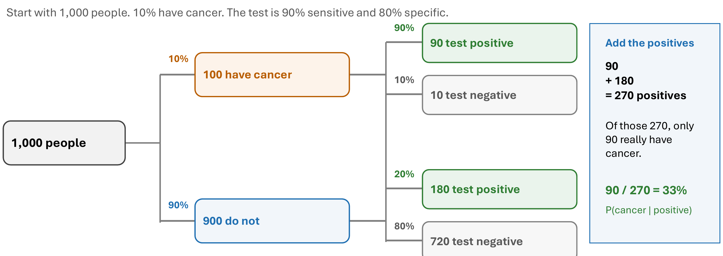
If an outcome can happen in two ways, through A or through not-A, add the two routes: each route is "chance of the cause times chance of the outcome given that cause". A tree diagram with a thousand people makes it concrete.
| Really has it (D) | Does not (¬D) | Read across the row | |
|---|---|---|---|
| Test positive (+) | true positive | false positive | positive predictive value \(P(D \mid +)\) |
| Test negative (−) | false negative | true negative | negative predictive value \(P(\neg D \mid -)\) |
| Read down the column | sensitivity \(P(+ \mid D)\) | specificity \(P(- \mid \neg D)\) |
Sensitivity reads down a column: given the person is ill, does the test catch it? Predictive value reads across a row: given a positive result, is the person ill? They can be 90% and 33% for the same test.
Recipe: P(evidence) through a tree
- Branch 1: \(P(H) \times P(E \mid H)\).
- Branch 2: \(P(\neg H) \times P(E \mid \neg H)\).
- \[ P(E) = \text{branch 1} + \text{branch 2} \]
New line makes 60% of boards (90% pass), old line 40% (80% pass): P(a board passes)?
- \[ P(N \cap P) = 0.60 \times 0.90 = 0.54 \]
- \[ P(O \cap P) = 0.40 \times 0.80 = 0.32 \]
- \[ P(P) = 0.54 + 0.32 = 0.86 \]
Fault 0.02, alarm on 95% of faulty cycles and 10% of clean ones: P(alarm)? And P(defective) for two machines (60% at 2%, 40% at 5%)
- \[ P(A) = 0.95 \times 0.02 + 0.10 \times 0.98 = 0.019 + 0.098 = 0.117 \]
- \[ P(D) = 0.6 \times 0.02 + 0.4 \times 0.05 = 0.012 + 0.020 = 0.032 \]
Bayes' rule: update a prior with evidence
Bayes' rule flips a conditional probability around: from "how likely is this evidence if the hypothesis is true" to "how likely is the hypothesis now that I have seen the evidence". The base rate does most of the work, so a positive test for a rare disease still usually means no disease.
L3 s86 says the word "win" appears in 10% of all emails, and L4 s42 repeats "0.1" in the Evidence line but uses 18% in the bullet and divides by 0.18. The 0.1 is impossible: it would give a posterior of \(0.14/0.1 = 1.4\). Since 20% of mail is spam and 70% of spam says "win", \(P(\text{"win"})\) must be at least 0.14; the 0.18 (with 5% of legitimate mail saying "win") is the consistent value. Posterior 78%.
Recipe
- Name \(H\) (the cause you are asked about) and \(E\) (what was observed).
- Write down \(P(H)\), \(P(E \mid H)\), \(P(E \mid \neg H)\).
- \[ P(E) = P(E \mid H)\,P(H) + P(E \mid \neg H)\,P(\neg H) \] (skip if \(P(E)\) is given)
- \[ P(H \mid E) = \frac{P(E \mid H)\,P(H)}{P(E)} \]
- Check it lies in \([0, 1]\) and that \(P(H \mid E) + P(\neg H \mid E) = 1\).
1% have the disease, 95% sensitivity, 2% false positives: P(disease | positive)
- \[ P(+) = 0.95 \times 0.01 + 0.02 \times 0.99 = 0.0095 + 0.0198 = 0.0293 \]
- \[ P(D \mid +) = \frac{0.0095}{0.0293} = 0.324 \]
- About 32%: better than the 8% with a 10% false-positive rate, still far from the 95% people expect.
10% of components defective; test says "Fail" for 90% of defective and 10% of good ones. P(D | Fail)?
- \[ P(D) = 0.10,\qquad P(F \mid D) = 0.90,\qquad P(F \mid D') = 0.10 \]
- \[ P(F) = 0.90 \times 0.10 + 0.10 \times 0.90 = 0.09 + 0.09 = 0.18 \]
- \[ P(D \mid F) = \frac{0.90 \times 0.10}{0.18} = 0.5 \]
- A "Fail" is a coin toss: the component is equally likely to be defective or good, because the 10% false-fail rate on the 90% of good parts produces as many fails as the true defectives.
Given that a board passed inspection, P(it came from the new line)?
- From the previous card, \(P(N \cap P) = 0.54\) and \(P(P) = 0.86\).
- \[ P(N \mid P) = \frac{0.54}{0.86} = 0.628 \]
- Check: \(P(O \mid P) = 0.32/0.86 = 0.372\); the two add to 1.
P(F) = 1%, P(unusual | F) = 80%, P(unusual) = 5%: P(fraud | unusual pattern)?
\(0.8 \times 0.01 / 0.05 = 0.16\). An unusual pattern raises the fraud probability from 1% to 16%.
P(fault | alarm), why it is not 0.95, and what happens on a less reliable machine
- \[ P(D \mid A) = \frac{0.95 \times 0.02}{0.117} = \frac{19}{117} = 0.162 \]
- 0.95 is \(P(A \mid D)\), the reverse conditional. Per 1,000 cycles: 19 genuine-fault alarms and 98 false alarms; only 19 of 117 alarms are faults.
- More frequent faults with the same alarm rates: \(P(D \mid A)\) increases, because a larger share of alarms now comes from faulty cycles.
Machine A 60% of parts at 2% defective, B 40% at 5%: P(B | defective)?
\(P(D) = 0.032\) (previous card), \(P(B \cap D) = 0.4 \times 0.05 = 0.020\), so \(P(B \mid D) = 0.020/0.032 = 0.625\).
Case study: Warner's randomised response
To ask an embarrassing question honestly, let a coin decide whether each student answers the real question or a harmless one. No single "yes" can be pinned on anyone, yet the class total still reveals the true proportion.
Total probability over the first toss: half the students answer Q1 and say yes with probability \(\pi\); half answer Q2 and say yes with probability \(\tfrac{1}{2}\). So \(P(\text{yes}) = \tfrac{1}{2}\pi + \tfrac{1}{2}\cdot\tfrac{1}{2}\).
Part 4
Exam toolkit
Match the wording to the rule, then check the arithmetic.
Which probability rule fits the wording?
| The question says… | Use | Card |
|---|---|---|
| equally likely outcomes, "a fair …" | count favourable / count all | Axioms |
| "not A", "other than" | \(1 - P(A)\) | Complement |
| "at least one" | \(1 - P(\text{none})\) | Complement |
| "A or B" | \(P(A) + P(B) - P(A \cap B)\); drop the last term if mutually exclusive | Addition |
| "A and B", independent | \(P(A)\,P(B)\) | Independence |
| "A and B", without replacement | \(P(A)\,P(B \mid A)\) | Conditional |
| "given that", "of those who" | \(P(A \mid B) = P(A \cap B)/P(B)\) | Conditional |
| are they independent? | compare \(P(A \cap B)\) with \(P(A)P(B)\), or \(P(B \mid A)\) with \(P(B)\) | Independence |
| exactly \(k\) of \(n\) in some order | \(\binom{n}{k}\) ways | Counting |
| overall probability of the evidence | \(\sum P(E \mid H_i)\,P(H_i)\) | Total probability |
| you know \(P(E \mid H)\) but want \(P(H \mid E)\) | \(P(E \mid H)P(H)/P(E)\) | Bayes |
Subtract the overlap in the addition rule. Mutually exclusive is not independent. \(P(A \mid B) \ne P(B \mid A)\): always write the denominator. Every probability must lie in \([0, 1]\) and a complete distribution must sum to 1; if yours does not, you added when you should have multiplied, or forgot an overlap.